The QUANTSELECT Procedure

This example is based on Surface Fitting with Many Noisy Variables in Chapter 25: The ADAPTIVEREG Procedure. This example shows how you can use the EFFECT statement to select a nonlinear surface model for a data set that contains many nuisance variables.

Consider a simulated data set that contains a response variable and 10 continuous predictors. Each continuous predictor is sampled independently from the uniform distribution . The true model of the artificial data set depends nonlinearly on two variables x1 and x2:

The values of the response variable are generated by adding errors from the standard normal distribution to the true model. The generating mechanism is adapted from Gu et al. (1990). The following statements create an artificial data set that contains 400 observations for the purpose of effect selection and 10,201 observations of missing response values for the purpose of prediction:

%let p=10;
data artificial;
   drop i;
   array x{&p};
   do i=1 to 400;
      do j=1 to &p;
         x{j} = ranuni(1);
      end;
      yTrain = 40*exp(8*((x1-0.5)**2+(x2-0.5)**2))/
          (exp(8*((x1-0.2)**2+(x2-0.7)**2))+
          exp(8*((x1-0.7)**2+(x2-0.2)**2)))+rannor(1);
      output;
   end;

   yTrain = .;
   do x1=0 to 1 by 0.01;
      do x2 = 0 to 1 by 0.01;
         y = 40*exp(8*((x1-0.5)**2+(x2-0.5)**2))/
             (exp(8*((x1-0.2)**2+(x2-0.7)**2))+
             exp(8*((x1-0.7)**2+(x2-0.2)**2)));
         output;
      end;
   end;
run;

The variables x3 through x10 are nuisance variables that can cause overfitting in your analysis. The following statements invoke the QUANTSELECT procedure to select effects, fit a model on the selected effects, and output the model predictions to an output data set Out:

%macro art;
   proc quantselect data=artificial algorithm=smooth;
      %do i=1 %to &p;
         effect sp&i = spline(x&i);
      %end;
      model yTrain =
         sp1 %do i=2 %to &p; |sp&i %end; @2/details=all;
      output out=Out p=pred;
   run;
%mend;

%art;

You can use the EFFECT statement to generate nonlinear effects and model a nonlinear surface. This example uses spline effects on variables and includes all the two-way interactions among these spline effects.

The ALGORITHM=SMOOTH option specifies the smoothing algorithm for model fitting. It takes approximately 2.8 seconds to select the model on a PC that has an Intel i7-2600 quad-core CPU and 64-bit Windows 7 Enterprise operation system. If you use the ALGORITHM=SIMPLEX option, which is default, it takes approximately 8.7 seconds for the same computation settings.

Output 96.4.1 shows the model information. By default, the effect selection method is the stepwise method, and the selection criterion is SBC for the SELECT=, CHOOSE=, and STOP= options. The default quantile level is 0.5 for median regression.

Output 96.4.2 shows the best 10 entry candidates at the selection step. You can see that sp1*sp2 is the most important effect, followed by sp1 and sp2.

Output 96.4.3 shows the selection summary.

The following statements produce a graph that shows both the true model and the fitted model:

ods graphics on;
data pred;
   set out;
   where yTrain=.;
run;

%let off0 = offsetmin=0 offsetmax=0;
%let off0 = xaxisopts=(&off0) yaxisopts=(&off0);
%let eopt = location=outside valign=top textattrs=graphlabeltext;
proc template;
   define statgraph surfaces;
      begingraph / designheight=360px;
         layout lattice/columns=2;
            layout overlay / &off0;
               entry "True Model" / &eopt;
               contourplotparm z=y y=x2 x=x1;
            endlayout;
            layout overlay / &off0;
               entry "Fitted Model" / &eopt;
               contourplotparm z=pred y=x2 x=x1;
            endlayout;
         endlayout;
      endgraph;
   end;
run;

proc sgrender data=pred template=surfaces;
run;

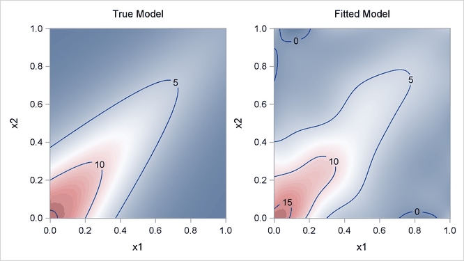
Output 96.4.4 displays surfaces for both the true model and the fitted model. You can see that the fitted model nicely approximates the underlying true model.

Output 96.4.4: True Model and Fitted Model