The PHREG Procedure
- Overview
-
Getting Started

-
SyntaxPROC PHREG StatementASSESS StatementBASELINE StatementBAYES StatementBY StatementCLASS StatementCONTRAST StatementEFFECT StatementESTIMATE StatementFREQ StatementHAZARDRATIO StatementID StatementLSMEANS StatementLSMESTIMATE StatementMODEL StatementOUTPUT StatementProgramming StatementsRANDOM StatementSTRATA StatementSLICE StatementSTORE StatementTEST StatementWEIGHT Statement
-
DetailsFailure Time DistributionTime and CLASS Variables UsagePartial Likelihood Function for the Cox ModelCounting Process Style of InputLeft-Truncation of Failure TimesThe Multiplicative Hazards ModelProportional Rates/Means Models for Recurrent EventsThe Frailty ModelProportional Subdistribution Hazards Model for Competing-Risks DataHazard RatiosNewton-Raphson MethodFirth’s Modification for Maximum Likelihood EstimationRobust Sandwich Variance EstimateTesting the Global Null HypothesisType 3 Tests and Joint TestsConfidence Limits for a Hazard RatioUsing the TEST Statement to Test Linear HypothesesAnalysis of Multivariate Failure Time DataModel Fit StatisticsSchemper-Henderson Predictive MeasureResidualsDiagnostics Based on Weighted ResidualsInfluence of Observations on Overall Fit of the ModelSurvivor Function EstimatorsCaution about Using Survival Data with Left TruncationEffect Selection MethodsAssessment of the Proportional Hazards ModelThe Penalized Partial Likelihood Approach for Fitting Frailty ModelsSpecifics for Bayesian AnalysisComputational ResourcesInput and Output Data SetsDisplayed OutputODS Table NamesODS Graphics
-
ExamplesStepwise RegressionBest Subset SelectionModeling with Categorical PredictorsFirth’s Correction for Monotone LikelihoodConditional Logistic Regression for m:n MatchingModel Using Time-Dependent Explanatory VariablesTime-Dependent Repeated Measurements of a CovariateSurvival CurvesAnalysis of ResidualsAnalysis of Recurrent Events DataAnalysis of Clustered DataModel Assessment Using Cumulative Sums of Martingale ResidualsBayesian Analysis of the Cox ModelBayesian Analysis of Piecewise Exponential ModelAnalysis of Competing-Risks Data
- References
Schemper-Henderson Predictive Measure
Measures of predictive accuracy of regression models quantify the extent to which covariates determine an individual outcome. Schemper and Henderson’s (2000) proposed predictive accuracy measure is defined as the difference between individual processes and the fitted survivor function.
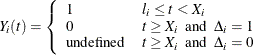
For the ith individual ( ), let
  and
and  be the left-truncation time, observed time, event indicator (1 for death and 0 for censored), and covariate vector, respectively.
If there is no delay entry, then
be the left-truncation time, observed time, event indicator (1 for death and 0 for censored), and covariate vector, respectively.
If there is no delay entry, then  . Let
. Let  be m distinct event times with
  deaths at
  . The survival process
  for the ith individual is
Let  be the Kaplan-Meier estimate of the survivor function (assuming no covariates). Let
  be the fitted survivor function with covariates
  , and if you specify TIES=EFRON, then is computed by the Efron method; otherwise, the Breslow estimate is used.
The predictive accuracy is defined as the difference between individual survival processes and the fitted survivor functions with ( )) or without () covariates between 0 and
  , the largest observed time. For each death time , define a mean absolute distance between the and the as
![\begin{eqnarray*} \hat{M}(t_{(j)}) & =& \frac{1}{n_ j} \sum _{i=1}^ n I(l_ i \le t_{(j)}) \biggl \{ I(X_ i>t_{(j)} \ge l_ i)(1-\hat{S}(t_{(j)}))+ \Delta _ i I(X_ i \leq t_{(j)})\hat{S}(t_{(j)}) \\ & & + ~ (1-\Delta _ i)I(X_ i \le t_{(j)}) \left[ (1-\hat{S}(t_{(j)}) )\frac{\hat{S}(t_{(j)})}{\hat{S}(X_ i)} +\hat{S}(t_{(j)}) \left(1 - \frac{\hat{S}(t_{(j)})}{\hat{S}(X_ i)} \right) \right] \biggr \} \end{eqnarray*}](images/statug_phreg0563.png)
where 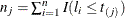 . Let
. Let  be defined similarly to
  , but with
  replaced by
  and
and  replaced by
  . Let
. Let  be the Kaplan-Meier estimate of the censoring or potential follow-up distribution, and let
![\[ w= \sum _{j=1}^ m \frac{d_ j}{\hat{G}(t_{(j)})} \]](images/statug_phreg0572.png)
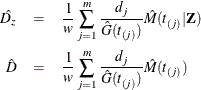
The overall estimator of the predictive accuracy with ( ) and without (
 ) covariates are weighted averages of and , respectively, given by
The explained variation by the Cox regression is
![\[ V = 100 \left(1- \frac{\hat{D}_ z}{\hat{D}}\right) \% \]](images/statug_phreg0576.png)
Because the predictive accuracy measures and are based on differences between individual survival processes and fitted survivor functions, a smaller value indicates a
better prediction. For this reason, and are also referred to as predictive inaccuracy measures.