The NLMIXED Procedure
-
Overview

-
Getting Started
-
Syntax
-
DetailsModeling Assumptions and NotationIntegral ApproximationsBuilt-in Log-Likelihood FunctionsHierarchical Model SpecificationOptimization AlgorithmsFinite-Difference Approximations of DerivativesHessian ScalingActive Set MethodsLine-Search MethodsRestricting the Step LengthComputational ProblemsCovariance MatrixPredictionComputational ResourcesDisplayed OutputODS Table Names
-
Examples
- References
Integral Approximations
An important part of the marginal maximum likelihood method described previously is the computation of the integral over the random effects. The default method in PROC NLMIXED for computing this integral is adaptive Gaussian quadrature as described in Pinheiro and Bates (1995). Another approximation method is the first-order method of Beal and Sheiner (1982, 1988). A description of these two methods follows.
Adaptive Gaussian Quadrature
A quadrature method approximates a given integral by a weighted sum over predefined abscissas for the random effects. A good
approximation can usually be obtained with an adequate number of quadrature points as well as appropriate centering and scaling
of the abscissas. Adaptive Gaussian quadrature for the integral over  centers the integral at the empirical Bayes estimate of , defined as the vector
  that minimizes
![\[ -\log \left[ p(\mb{y}_ i | \mb{X}_ i,\bphi , \mb{u}_ i) q(\mb{u}_ i | \bxi ) \right] \]](images/statug_nlmixed0145.png)
with  and
and  set equal to their current estimates. The final Hessian matrix from this optimization can be used to scale the quadrature
abscissas.
set equal to their current estimates. The final Hessian matrix from this optimization can be used to scale the quadrature
abscissas.
Suppose 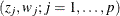 denote the standard Gauss-Hermite abscissas and weights (Golub and Welsch 1969, or Table 25.10 of Abramowitz and Stegun 1972). The adaptive Gaussian quadrature integral approximation is as follows:
![\begin{align*} \lefteqn{ \int p(\mb{y}_ i | \mb{X}_ i, \bphi , \mb{u}_ i) q(\mb{u}_ i | \bxi ) d \mb{u}_ i \approx } \\ & 2^{r/2} \left| \bGamma (\mb{X}_ i,\btheta ) \right|^{-1/2} \sum _{j_1=1}^ p \cdots \sum _{j_ r=1}^ p \left[ p(\mb{y}_ i | \mb{X}_ i, \bphi , \mb{a}_{j_1,\ldots ,j_ r}) q(\mb{a}_{j_1,\ldots ,j_ r} | \bxi ) \prod _{k=1}^ r w_{j_ k} \exp {z^2_{j_ k}} \right] \\ \end{align*}](images/statug_nlmixed0147.png)
where r is the dimension of  ,
,  is the Hessian matrix from the empirical Bayes minimization,
  is a vector with elements
  , and
, and
![\[ \mb{a}_{j_1,\ldots ,j_ r} = \widehat{\mb{u}}_ i + 2^{1/2} \bGamma (\mb{X}_ i,\btheta )^{-1/2} \mb{z}_{j_1,\ldots ,j_ r} \]](images/statug_nlmixed0151.png)
PROC NLMIXED selects the number of quadrature points adaptively by evaluating the log-likelihood function at the starting values of the parameters until two successive evaluations have a relative difference less than the value of the QTOL= option. The specific search sequence is described under the QFAC= option. Using the QPOINTS= option, you can adjust the number of quadrature points p to obtain different levels of accuracy. Setting p = 1 results in the Laplacian approximation as described in: Beal and Sheiner (1992); Wolfinger (1993); Vonesh (1992, 1996); Vonesh and Chinchilli (1997); Wolfinger and Lin (1997).
The NOAD
option in the PROC NLMIXED
statement requests nonadaptive Gaussian quadrature. Here all are set equal to zero, and the Cholesky root of the estimated variance matrix of the random effects is substituted for  in the preceding expression for
  . In this case derivatives are computed using the algorithm of Smith (1995). The NOADSCALE
option requests the same scaling substitution but with the empirical Bayes . When there is one RANDOM
statement, the dimension of is the number of random effects that are specified in that RANDOM
statement. For nested multilevel nonlinear mixed models, the dimension of could increase significantly. In this case, the dimension of is equal to the sum of all nested subjects times the corresponding random-effects dimension. For example, consider a three-level
nested nonlinear mixed model that contains s first-level subjects, where each first-level subject has
. In this case derivatives are computed using the algorithm of Smith (1995). The NOADSCALE
option requests the same scaling substitution but with the empirical Bayes . When there is one RANDOM
statement, the dimension of is the number of random effects that are specified in that RANDOM
statement. For nested multilevel nonlinear mixed models, the dimension of could increase significantly. In this case, the dimension of is equal to the sum of all nested subjects times the corresponding random-effects dimension. For example, consider a three-level
nested nonlinear mixed model that contains s first-level subjects, where each first-level subject has  second-level subjects that are nested within and
  third-level subjects that are nested within each combination of first-level subject i and second-level subject j. Then, based on notation in the previous section,
  . Suppose
  is the random-effects dimension at level i. Then the dimension of , denoted as r, can be computed as
  . Hence the joint estimation of is more costly.
When only one RANDOM statement is specified for the model, by default PROC NLMIXED uses Newton-Raphson optimization for empirical Bayes minimization of random effects for each subject. If you specify the EBOPT option in the PROC NLMIXED statement, then the procedure uses Newton-Raphson ridge optimization. But when multiple RANDOM statements are specified, quasi-Newton optimization is used for the empirical Bayes minimization of random effects for each subject. Therefore, all the options that are related to the Newton-Raphson method (such as the EBOPT , EBSSFRAC= , EBSSTOL= , EBSTEPS= , EBSUBSTEPS= , and EBTOL= options) are ignored.
PROC NLMIXED computes the derivatives of the adaptive Gaussian quadrature approximation when carrying out the default dual quasi-Newton optimization. For nested multilevel nonlinear mixed models, PROC NLMIXED does not explicitly compute these derivatives. In this case, it ignores the EMPIRICAL and SUBGRADIENT= options in the PROC NLMIXED statement. Also, nested multilevel nonlinear mixed models use METHOD= GAUSS only. In addition to these changes, for nested multilevel nonlinear mixed models, the default values of GTOL and ABSGTOL are changed to 1E–6 and 1E–3, respectively.
First-Order Method
Another integral approximation available in PROC NLMIXED is the first-order method of Beal and Sheiner (1982, 1988) and Sheiner and Beal (1985). This approximation is used only in the case where  is normal—that is,
![\begin{align*} p(\mb{y}_ i | \mb{X}_ i, \bphi , \mb{u}_ i) & = (2 \pi )^{-n_ i/2} \left| \mb{R}_ i(\mb{X}_ i,\bphi ) \right| ^{-1/2} \\ & \exp \left\{ -(1/2) \left[ \mb{y}_ i - \mb{m}_ i(\mb{X}_ i,\bphi ,\mb{u}_ i) \right]^\prime \mb{R}_ i(\mb{X}_ i,\bphi )^{-1} \left[ \mb{y}_ i - \mb{m}_ i(\mb{X}_ i,\bphi ,\mb{u}_ i) \right] \right\} \end{align*}](images/statug_nlmixed0159.png)
where  is the dimension of
  ,
,  is a diagonal variance matrix, and
  is the conditional mean vector of .
The first-order approximation is obtained by expanding  with a one-term Taylor series expansion about
  , resulting in the approximation
![\begin{align*} p(\mb{y}_ i | \mb{X}_ i, \bphi , \mb{u}_ i) & \approx (2 \pi )^{-n_ i/2} \left| \mb{R}_ i(\mb{X}_ i,\bphi ) \right| ^{-1/2} \\ & \exp \left( -(1/2) \left[ \mb{y}_ i - \mb{m}_ i(\mb{X}_ i,\bphi ,\mb{0}) - \mb{Z}_ i(\mb{X}_ i,\bphi ) \mb{u}_ i \right]^\prime \right. \\ & \left. \vphantom {-(1/2) \left[ \mb{y}_ i - \mb{m}_ i(\mb{X}_ i,\bphi ,\mb{0}) - \mb{Z}_ i(\mb{X}_ i,\bphi ) \mb{u}_ i \right]^\prime }\mb{R}_ i(\mb{X}_ i,\bphi )^{-1} \left[ \mb{y}_ i - \mb{m}_ i(\mb{X}_ i,\bphi ,\mb{0}) - \mb{Z}_ i(\mb{X}_ i,\bphi ) \mb{u}_ i \right] \right) \end{align*}](images/statug_nlmixed0165.png)
where  is the Jacobian matrix
  evaluated at .
Assuming that  is normal with mean
  and variance matrix
  , the first-order integral approximation is computable in closed form after completing the square:
![\begin{align*} \int p(\mb{y}_ i | \mb{X}_ i, \bphi , \mb{u}_ i) q(\mb{u}_ i | \bxi )\, d \mb{u}_ i & \approx (2 \pi )^{-n_ i/2} \left| \mb{V}_ i(\mb{X}_ i,\btheta ) \right|^{-1/2} \\ & \exp \left( -(1/2) \left[ \mb{y}_ i - \mb{m}_ i(\mb{X}_ i,\bphi ,\mb{0}) \right]^\prime \mb{V}_ i(\mb{X}_ i,\btheta )^{-1} \left[ \mb{y}_ i - \mb{m}_ i(\mb{X}_ i,\bphi ,\mb{0}) \right] \right) \end{align*}](images/statug_nlmixed0171.png)
where  . The resulting approximation for
  is then minimized over
 ![$\btheta = [\bphi , \bxi ]$](images/statug_nlmixed0118.png) to obtain the first-order estimates. PROC NLMIXED uses finite-difference derivatives of the first-order integral approximation
when carrying out the default dual quasi-Newton optimization.
to obtain the first-order estimates. PROC NLMIXED uses finite-difference derivatives of the first-order integral approximation
when carrying out the default dual quasi-Newton optimization.