The HPGENSELECT Procedure
-
Overview

- Getting Started
-
Syntax
-
DetailsMissing ValuesExponential Family DistributionsResponse DistributionsResponse Probability Distribution FunctionsLog-Likelihood FunctionsThe LASSO Method of Model SelectionUsing Validation and Test DataComputational Method: MultithreadingChoosing an Optimization AlgorithmDisplayed OutputODS Table Names
-
Examples
- References
The LASSO Method of Model Selection
LASSO Selection
The HPGENSELECT procedure implements the group LASSO method, which is described in the section Group LASSO Selection. This section provides some background about the LASSO method that you need in order to understand the group LASSO method.
LASSO (least absolute shrinkage and selection operator) selection arises from a constrained form of ordinary least squares
regression in which the sum of the absolute values of the regression coefficients is constrained to be smaller than a specified
parameter. More precisely, let 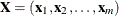 denote the matrix of covariates, and let
  denote the response. Then for a given parameter t, the LASSO regression coefficients
 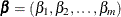 are the solution to the constrained least squares problem
![\[ \min ||\mb{y}-\bX \bbeta ||^2 \qquad \mbox{subject to} \quad \sum _{j=1}^{m} | \beta _ j | \leq t \]](images/statug_hpgenselect0128.png)
For generalized linear models, the LASSO regression coefficients are the solution to the constrained optimization problem
![\[ \min \{ -L(\bmu ;\mb{y})\} \qquad \mbox{subject to} \quad \sum _{j=1}^{m} | \beta _ j | \leq t \]](images/statug_hpgenselect0129.png)
where L is the log-likelihood function defined in the section Log-Likelihood Functions.
Provided that the LASSO parameter t is small enough, some of the regression coefficients will be exactly zero. Hence, you can view the LASSO method as selecting a subset of the regression coefficients for each LASSO parameter. By increasing the LASSO parameter in discrete steps, you obtain a sequence of regression coefficients for which the nonzero coefficients at each step correspond to selected parameters. For more information about the LASSO method, see, for example, Hastie, Tibshirani, and Friedman (2009).
Group LASSO Selection
The group LASSO method, proposed by Yuan and Lin (2006), is a variant of LASSO that is specifically designed for models defined in terms of effects that have multiple degrees of freedom, such as the main effects of CLASS variables, and interactions between CLASS variables. If all effects in the model are continuous, then the group LASSO method is the same as the LASSO method.
Recall that LASSO selection depends on solving a constrained optimization problem of the form
In this formulation, individual parameters can be included or excluded from the model independently, subject only to the
overall constraint. In contrast, the group LASSO method uses a constraint that forces all parameters corresponding to the
same effect to be included or excluded simultaneously. For a model that has k effects, let  be the group of linear coefficients that correspond to effect j in the model. Then group LASSO depends on solving a constrained optimization problem of the form
![\[ \min \{ -L(\bmu ;\mb{y})\} \qquad \mbox{subject to} \quad \sum _{j=1}^{k} \sqrt {|G_ j|} ||\beta _{G_ j}|| \leq t \]](images/statug_hpgenselect0131.png)
where  is the number of parameters that correspond to effect j, and
  denotes the Euclidean norm of the parameters ,
![\[ ||\beta _{G_ j}||= \sqrt {\sum _{i=1}^{G_ j} \beta _ i^2} \]](images/statug_hpgenselect0134.png)
That is, instead of constraining the sum of the absolute value of individual parameters, group LASSO constrains the Euclidean norm of groups of parameters, where groups are defined by effects.
You can write the group LASSO method in the equivalent Lagrangian form, which is an example of a penalized log-likelihood function:
![\[ \min \{ -L(\bmu ;\mb{y})\} + \lambda \sum _{j=1}^{k} \sqrt {|G_ j|} ||\beta _{G_ j} || \]](images/statug_hpgenselect0135.png)
The weight  was suggested by Yuan and Lin (2006) in order to take the size of the group into consideration in group LASSO.
Unlike LASSO for linear models, group LASSO does not allow a piecewise linear constant solution path as generated by a LAR
algorithm. Instead, the method proposed by Nesterov (2013) is adopted to solve the Lagrangian form of the group LASSO problem that corresponds to a prespecified regularization parameter
 . Nesterov’s method is known to have an optimal convergence rate for first-order black box optimization. Because the optimal
is usually unknown, a series of regularization parameters
. Nesterov’s method is known to have an optimal convergence rate for first-order black box optimization. Because the optimal
is usually unknown, a series of regularization parameters  is employed, where
  is a positive value less than 1. You can specify by using the LASSORHO= option in the PROC HPGENSELECT
statement; the default value is
is a positive value less than 1. You can specify by using the LASSORHO= option in the PROC HPGENSELECT
statement; the default value is  . In the ith step of group LASSO selection, the value that is used for is
  .
.
A unique feature of the group LASSO method is that it does not necessarily add or remove precisely one effect at each step of the process. This is different from the forward, stepwise, and backward selection methods.
As with the other selection methods that PROC HPGENSELECT supports, you can specify a criterion to choose among the models at each step of the group LASSO algorithm by using the CHOOSE= option in the SELECTION statement. You can also specify a stopping criterion by using the STOP= option in the SELECTION statement. If you do not specify either the CHOOSE= or STOP= option, the model at the last LASSO step is chosen as the selected model, and parameter estimates are reported for this model. If you request an output data set by using an OUTPUT statement, these parameter estimates are used to compute predicted values in the output data set.
For more information, see the discussion in the section SELECTION Statement in SAS/STAT 14.1 User's Guide: High-Performance Procedures.
The model degrees of freedom that PROC HPGENSELECT uses at any step of the LASSO are simply the number of nonzero regression coefficients in the model at that step. Efron et al. (2004) cite empirical evidence for doing this but do not give any mathematical justification for this choice.
Some distributions involve a dispersion parameter (the parameter  in the expressions for the log likelihood), and in the case of the Tweedie distribution, a power parameter. These parameters
are not estimated by the LASSO optimization algorithm, and are set to either the default value or a value that you specify.
You can use the MODEL statement options PHI= to set the dispersion to a fixed value and P= to set the Tweedie power parameter
to a fixed value.
in the expressions for the log likelihood), and in the case of the Tweedie distribution, a power parameter. These parameters
are not estimated by the LASSO optimization algorithm, and are set to either the default value or a value that you specify.
You can use the MODEL statement options PHI= to set the dispersion to a fixed value and P= to set the Tweedie power parameter
to a fixed value.