The ADAPTIVEREG Procedure

Example 25.4 Nonparametric Poisson Model for Mackerel Egg Density
This example demonstrates how you can use PROC ADAPTIVEREG to fit a nonparametric Poisson regression model.
The example concerns a study of mackerel egg density. The data are a subset of the 1992 mackerel egg survey conducted over the Porcupine Bank west of Ireland. The survey took place in the peak spawning area. Scientists took samples by hauling a net up from deep sea to the sea surface. Then they counted the number of spawned mackerel eggs and used other geographic information to estimate the sizes and distributions of spawning stocks. The data set is used as an example in Bowman and Azzalini (1997).
The following SAS DATA step creates the data set Mackerel. This data set contains 634 observations and five variables. The response variable Egg_Count is the number of mackerel eggs collected from each sampling net. Longitude and Latitude are the location values in degrees east and north, respectively, of each sample station. Net_Area is the area of the sampling net in square meters. Depth records the sea bed depth in meters at the sampling location. And Distance is the distance in geographic degrees from the sample location to the continental shelf edge.
title 'Mackerel Egg Density Study';
data Mackerel;
   input Egg_Count Longitude Latitude  Net_Area Depth Distance;
   datalines;
   0     -4.65     44.57     0.242    4342    0.8395141177
   0     -4.48     44.57     0.242    4334    0.8591926336
   0      -4.3     44.57     0.242    4286    0.8930152895
   1     -2.87     44.02     0.242    1438    0.3956408691
   4     -2.07     44.02     0.242     166    0.0400088237
   3     -2.13     44.02     0.242     460    0.0974234463
   0     -2.27     44.02     0.242     810    0.2362566569

   ... more lines ...

  22     -4.22     46.25      0.19     205    0.1181120828
  21     -4.28     46.25      0.19     237     0.129990854
   0     -4.73     46.25      0.19    2500    0.3346500536
   5     -4.25     47.23      0.19     114     0.718192582
   3     -3.72     47.25      0.19     100    0.9944669778
   0     -3.25     47.25      0.19      64    1.2639918431
;
The response values are counts, so the Poisson distribution might be a reasonable model. The study of interest is the mackerel egg density, which can be formed as
![\[ \mathrm{density} = E(\mathrm{count})/\mathrm{net\_ area} \]](images/statug_adaptivereg0124.png)
This is equivalent to a Poisson regression with the response variable Egg_Count and an offset variable  and other covariates.
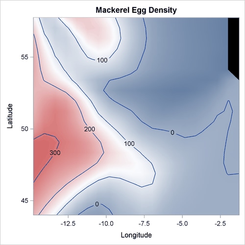
The following statements produce the plot of the mackerel egg density with respect to the sampling station location:
data temp;
   set mackerel;
   density = egg_count/net_area;
run;
%let off0 = offsetmin=0 offsetmax=0 linearopts=(thresholdmin=0 thresholdmax=0);
proc template;
   define statgraph surface;
      dynamic _title _z;
      begingraph / designwidth=defaultDesignHeight;
         entrytitle _title;
         layout overlay / xaxisopts=(&off0) yaxisopts=(&off0);
            contourplotparm z=_z y=latitude x=longitude / gridded=FALSE;
         endlayout;
      endgraph;
   end;
run;

proc sgrender data=temp template=surface;
   dynamic _title='Mackerel Egg Density' _z='density';
run;
Output 25.4.1 displays the mackerel egg density in the sampling area. The black hole in the upper right corner is due to missing values in that area.
Output 25.4.1: Mackerel Egg Density
In this example, the dependent variable is the mackerel egg counts, the independent variables are the geographical information about each of the sampling stations, and the logarithm of the sampling area is the offset variable. The following statements fit the nonparametric Poisson regression model:
data mackerel;
   set mackerel;
   log_net_area = log(net_area);
run;
proc adaptivereg data=mackerel;
   model egg_count = longitude latitude depth distance
                      / offset=log_net_area dist=poisson;
   output out=mackerelout p(ilink);
run;
Output 25.4.2 lists basic model information such as the offset variable, distribution, and link function.
Output 25.4.2: Model Information
Output 25.4.3 lists fit statistics for the final model.
Output 25.4.3: Fit Statistics
The final model consists of basis functions and interactions between basis functions of three geographic variables. Output 25.4.4 lists seven functional components of the final model, including three one-way spline transformations and four two-way spline interactions.
Output 25.4.4: ANOVA Decomposition
| ANOVA Decomposition | ||||
|---|---|---|---|---|
| Functional Component |
Number of Bases |
DF | Change If Omitted | |
| Lack of Fit | GCV | |||
| Longitude | 3 | 6 | 2035.77 | 3.3216 |
| Depth | 1 | 2 | 420.59 | 0.6780 |
| Latitude | 1 | 2 | 265.05 | 0.4104 |
| Longitude Latitude | 2 | 4 | 199.17 | 0.2496 |
| Depth Distance | 3 | 6 | 552.75 | 0.8030 |
| Depth Latitude | 2 | 4 | 680.45 | 1.0723 |
| Depth Longitude | 2 | 4 | 415.77 | 0.6198 |
The "Variable Importance" table in Output 25.4.5 displays the relative variable importance among the four variables. Longitude is the most important one.
Output 25.4.5: Variable Importance
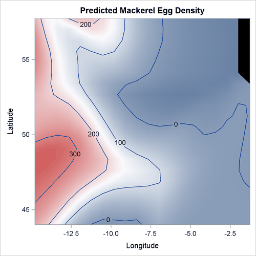
The following steps create and display in Output 25.4.6 the predicted mackerel egg density over the spawning area.
data mackplot;
   set mackerelout;
   density = pred / net_area;
run;
proc sgrender data=mackplot template=surface;
   dynamic _title='Predicted Mackerel Egg Density'
           _z='density';
run;
Output 25.4.6: Predicted Mackerel Egg Density