The GLM Procedure

Analysis of covariance combines some of the features of both regression and analysis of variance. Typically, a continuous variable (the covariate) is introduced into the model of an analysis-of-variance experiment.

Data in the following example are selected from a larger experiment on the use of drugs in the treatment of leprosy (Snedecor and Cochran, 1967, p. 422).

Variables in the study are as follows:

Ten patients are selected for each treatment (Drug), and six sites on each patient are measured for leprosy bacilli.

The covariate (a pretreatment score) is included in the model for increased precision in determining the effect of drug treatments on the posttreatment count of bacilli.

The following statements create the data set, perform a parallel-slopes analysis of covariance with PROC GLM, and compute Drug LS-means. These statements produce Output 45.4.1 and Output 45.4.2.

data DrugTest;
   input Drug $ PreTreatment PostTreatment @@;
   datalines;
A 11  6   A  8  0   A  5  2   A 14  8   A 19 11
A  6  4   A 10 13   A  6  1   A 11  8   A  3  0
D  6  0   D  6  2   D  7  3   D  8  1   D 18 18
D  8  4   D 19 14   D  8  9   D  5  1   D 15  9
F 16 13   F 13 10   F 11 18   F  9  5   F 21 23
F 16 12   F 12  5   F 12 16   F  7  1   F 12 20
;

proc glm data=DrugTest;
   class Drug;
   model PostTreatment = Drug PreTreatment / solution;
   lsmeans Drug / stderr pdiff cov out=adjmeans;
run;

proc print data=adjmeans;
run;

This model assumes that the slopes relating posttreatment scores to pretreatment scores are parallel for all drugs. You can check this assumption by including the class-by-covariate interaction, Drug*PreTreatment, in the model and examining the ANOVA test for the significance of this effect. This extra test is omitted in this example, but it is insignificant, justifying the equal-slopes assumption.

In Output 45.4.3, the Type I SS for Drug (293.6) gives the between-drug sums of squares that are obtained for the analysis-of-variance model PostTreatment=Drug. This measures the difference between arithmetic means of posttreatment scores for different drugs, disregarding the covariate. The Type III SS for Drug (68.5537) gives the Drug sum of squares adjusted for the covariate. This measures the differences between Drug LS-means, controlling for the covariate. The Type I test is highly significant (p = 0.001), but the Type III test is not. 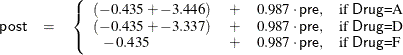This indicates that, while there is a statistically significant difference between the arithmetic drug means, this difference is reduced to below the level of background noise when you take the pretreatment scores into account. From the table of parameter estimates, you can derive the least squares predictive formula model for estimating posttreatment score based on pretreatment score and drug:

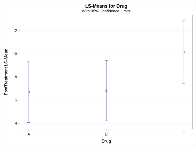
Output 45.4.4 displays the LS-means, which are, in a sense, the means adjusted for the covariate. The STDERR option in the LSMEANS statement causes the standard error of the LS-means and the probability of getting a larger t value under the hypothesis to be included in this table as well. Specifying the PDIFF option causes all probability values for the hypothesis to be displayed, where the indexes i and j are numbered treatment levels.

The OUT= and COV options in the LSMEANS statement create a data set of the estimates, their standard errors, and the variances and covariances of the LS-means, which is displayed in Output 45.4.5.

The new graphical features of PROC GLM enable you to visualize the fitted analysis of covariance model. The following statements enable ODS Graphics by specifying the ODS GRAPHICS statement and then fit an analysis-of-covariance model with LS-means for Drug.

ods graphics on;

proc glm data=DrugTest plot=meanplot(cl);
   class Drug;
   model PostTreatment = Drug PreTreatment;
   lsmeans Drug / pdiff;
run;

ods graphics off;

With graphics enabled, the GLM procedure output includes an analysis-of-covariance plot, as in Output 45.4.6. The LSMEANS statement produces a plot of the LS-means; the SAS statements previously shown use the PLOTS= MEANPLOT(CL) option to add confidence limits for the individual LS-means, shown in Output 45.4.7. If you also specify the PDIFF option in the LSMEANS statement, the output also includes a plot appropriate for the type of LS-mean differences computed. In this case, the default is to compare all LS-means with each other pairwise, so the plot is a "diffogram" or "mean-mean scatter plot" (Hsu, 1996), as in Output 45.4.8. For general information about ODS Graphics, see Chapter 21: Statistical Graphics Using ODS. For specific information about the graphics available in the GLM procedure, see the section ODS Graphics.

Output 45.4.6: Analysis of Covariance Plot of PostTreatment Score by Drug and PreTreatment Score

Output 45.4.7: LS-Means for PostTreatment Score by Drug

Output 45.4.8: Plot of Differences between Drug LS-Means for PostTreatment Scores

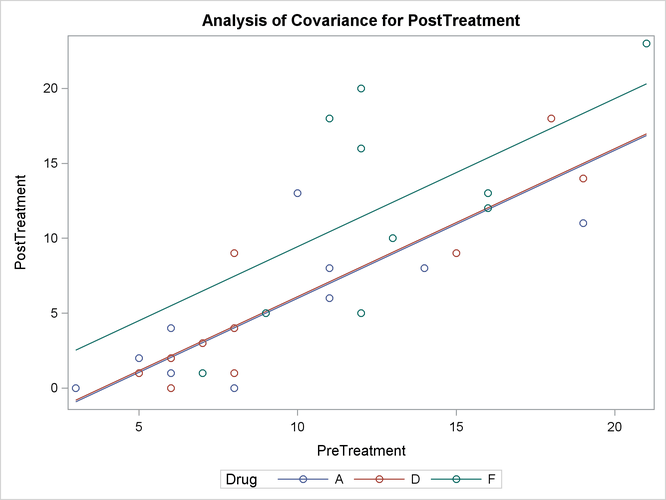
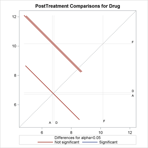
The analysis of covariance plot Output 45.4.6 makes it clear that the control (drug F) has higher posttreatment scores across the range of pretreatment scores, while the fitted models for the two antibiotics (drugs A and D) nearly coincide. Similarly, while the diffogram Output 45.4.7 indicates that none of the LS-mean differences are significant at the 5% level, the difference between the LS-means for the two antibiotics is much closer to zero than the differences between either one and the control.