The GLM Procedure

This example uses data from Kutner (1974, p. 98) to illustrate a two-way analysis of variance. The original data source is Afifi and Azen (1972, p. 166). These statements produce Output 45.3.1 and Output 45.3.2.

title 'Unbalanced Two-Way Analysis of Variance';
data a;
   input drug disease @;
   do i=1 to 6;
      input y @;
      output;
   end;
   datalines;
1 1 42 44 36 13 19 22
1 2 33  . 26  . 33 21
1 3 31 -3  . 25 25 24
2 1 28  . 23 34 42 13
2 2  . 34 33 31  . 36
2 3  3 26 28 32  4 16
3 1  .  .  1 29  . 19
3 2  . 11  9  7  1 -6
3 3 21  1  .  9  3  .
4 1 24  .  9 22 -2 15
4 2 27 12 12 -5 16 15
4 3 22  7 25  5 12  .
;

proc glm;
   class drug disease;
   model y=drug disease drug*disease / ss1 ss2 ss3 ss4;
run;

Note the differences among the four types of sums of squares. The Type I sum of squares for drug essentially tests for differences between the expected values of the arithmetic mean response for different drugs, unadjusted for the effect of disease. By contrast, the Type II sum of squares for drug measures the differences between arithmetic means for each drug after adjusting for disease. The Type III sum of squares measures the differences between predicted drug means over a balanced drugdisease population—that is, between the LS-means for drug. Finally, the Type IV sum of squares is the same as the Type III sum of squares in this case, since there are data for every drug-by-disease combination.

No matter which sum of squares you prefer to use, this analysis shows a significant difference among the four drugs, while the disease effect and the drug-by-disease interaction are not significant. As the previous discussion indicates, Type III sums of squares correspond to differences between LS-means, so you can follow up the Type III tests with a multiple-comparison analysis of the drug LS-means. Since the GLM procedure is interactive, you can accomplish this by submitting the following statements after the previous ones that performed the ANOVA.

   lsmeans drug / pdiff=all adjust=tukey;
run;

Both the LS-means themselves and a matrix of adjusted p-values for pairwise differences between them are displayed; see Output 45.3.3 and Output 45.3.4.

The multiple-comparison analysis shows that drugs 1 and 2 have very similar effects, and that drugs 3 and 4 are also insignificantly different from each other. Evidently, the main contribution to the significant drug effect is the difference between the 1/2 pair and the 3/4 pair.

If ODS Graphics is enabled for the previous analysis, GLM also displays three additional plots by default:

The following statements reproduce the previous analysis with ODS Graphics enabled. Additionally, the PLOTS= MEANPLOT(CL) option specifies that confidence limits for the LS-means should also be displayed in the mean plot. The graphical results are shown in Output 45.3.5 through Output 45.3.7.

ods graphics on;
proc glm plot=meanplot(cl);
   class drug disease;
   model y=drug disease drug*disease;
   lsmeans drug / pdiff=all adjust=tukey;
run;
ods graphics off;

Output 45.3.5: Plot of Response by Drug and Disease

Output 45.3.6: Plot of Response LS-Means for Drug

Output 45.3.7: Plot of Response LS-Mean Differences for Drug

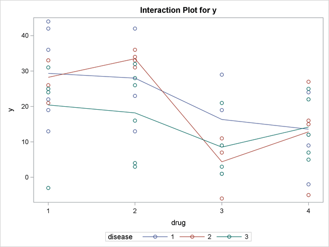
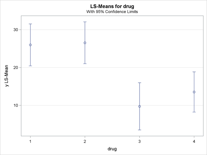
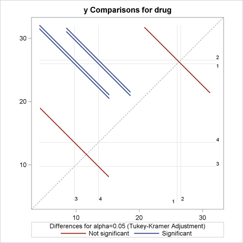
The significance of the drug differences is difficult to discern in the original data, as displayed in Output 45.3.5, but the plot of just the LS-means and their individual confidence limits in Output 45.3.6 makes it clearer. Finally, Output 45.3.7 indicates conclusively that the significance of the effect of drug is due to the difference between the two drug pairs (1, 2) and (3, 4).