The GLM Procedure
-
Overview

-
Getting Started
-
Syntax
-
DetailsStatistical Assumptions for Using PROC GLMSpecification of EffectsUsing PROC GLM InteractivelyParameterization of PROC GLM ModelsHypothesis Testing in PROC GLMEffect Size Measures for F Tests in GLMAbsorptionSpecification of ESTIMATE ExpressionsComparing GroupsMultivariate Analysis of VarianceRepeated Measures Analysis of VarianceRandom-Effects AnalysisMissing ValuesComputational ResourcesComputational MethodOutput Data SetsDisplayed OutputODS Table NamesODS Graphics
-
ExamplesRandomized Complete Blocks with Means Comparisons and ContrastsRegression with Mileage DataUnbalanced ANOVA for Two-Way Design with InteractionAnalysis of CovarianceThree-Way Analysis of Variance with ContrastsMultivariate Analysis of VarianceRepeated Measures Analysis of VarianceMixed Model Analysis of Variance with the RANDOM StatementAnalyzing a Doubly Multivariate Repeated Measures DesignTesting for Equal Group VariancesAnalysis of a Screening Design
- References
When comparing more than two means, an ANOVA F test tells you whether the means are significantly different from each other, but it does not tell you which means differ from which other means. Multiple-comparison procedures (MCPs), also called mean separation tests, give you more detailed information about the differences among the means. The goal in multiple comparisons is to compare the average effects of three or more "treatments" (for example, drugs, groups of subjects) to decide which treatments are better, which ones are worse, and by how much, while controlling the probability of making an incorrect decision. A variety of multiple-comparison methods are available with the MEANS and LSMEANS statement in the GLM procedure.
The following classification is due to Hsu (1996). Multiple-comparison procedures can be categorized in two ways: by the comparisons they make and by the strength of inference they provide. With respect to which comparisons are made, the GLM procedure offers two types:
-
comparisons between all pairs of means
-
comparisons between a control and all other means
The strength of inference says what can be inferred about the structure of the means when a test is significant; it is related to what type of error rate the MCP controls. MCPs available in the GLM procedure provide one of the following types of inference, in order from weakest to strongest:
-
Individual: differences between means, unadjusted for multiplicity
-
Inhomogeneity: means are different
-
Inequalities: which means are different
-
Intervals: simultaneous confidence intervals for mean differences
Methods that control only individual error rates are not true MCPs at all. Methods that yield the strongest level of inference, simultaneous confidence intervals, are usually preferred, since they enable you not only to say which means are different but also to put confidence bounds on how much they differ, making it easier to assess the practical significance of a difference. They are also less likely to lead nonstatisticians to the invalid conclusion that nonsignificantly different sample means imply equal population means. Interval MCPs are available for both arithmetic means and LS-means via the MEANS and LSMEANS statements, respectively.[29]
Table 45.11 and Table 45.12 display MCPs available in PROC GLM for all pairwise comparisons and comparisons with a control, respectively, along with associated strength of inference and the syntax (when applicable) for both the MEANS and the LSMEANS statements.
Table 45.11: Multiple-Comparison Procedures for All Pairwise Comparisons
|
Strength of |
Syntax |
||
|---|---|---|---|
|
Method |
Inference |
MEANS |
LSMEANS |
|
Student’s t |
Individual |
||
|
Duncan |
Individual |
||
|
Student-Newman-Keuls |
Inhomogeneity |
||
|
REGWQ |
Inequalities |
||
|
Tukey-Kramer |
Intervals |
||
|
Bonferroni |
Intervals |
||
|
Sidak |
Intervals |
||
|
Scheffé |
Intervals |
||
|
SMM |
Intervals |
||
|
Gabriel |
Intervals |
||
|
Simulation |
Intervals |
||
Table 45.12: Multiple-Comparison Procedures for Comparisons with a Control
|
Strength of |
Syntax |
||
|---|---|---|---|
|
Method |
Inference |
MEANS |
LSMEANS |
|
Student’s t |
Individual |
||
|
Dunnett |
Intervals |
PDIFF= CONTROL ADJUST=DUNNETT |
|
|
Bonferroni |
Intervals |
PDIFF= CONTROL ADJUST=BON |
|
|
Sidak |
Intervals |
PDIFF= CONTROL ADJUST=SIDAK |
|
|
Scheffé |
Intervals |
PDIFF= CONTROL ADJUST=SCHEFFE |
|
|
SMM |
Intervals |
PDIFF= CONTROL ADJUST=SMM |
|
|
Simulation |
Intervals |
PDIFF= CONTROL ADJUST=SIMULATE |
|
Note: One-sided Dunnett’s tests are also available from the MEANS statement with the DUNNETTL and DUNNETTU options and from the LSMEANS statement with PDIFF= CONTROLL and PDIFF= CONTROLU.
A note concerning the ODS tables for the results of the PDIFF or TDIFF options in the LSMEANS statement: The p/t-values for differences are displayed in columns of the LSMeans table for PDIFF /TDIFF =CONTROL or PDIFF /TDIFF =ANOM, and for PDIFF /TDIFF =ALL when there are only two LS-means. Otherwise (for PDIFF /TDIFF =ALL when there are more than two LS-means), the p/t-values for differences are displayed in a separate table called Diff.
Details of these multiple comparison methods are given in the following sections.
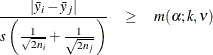
All the methods discussed in this section depend on the standardized pairwise differences ![]() , where the parts of this expression are defined as follows:
, where the parts of this expression are defined as follows:
-
i and j are the indices of two groups
-
 and
and  are the means or LS-means for groups i and j
-
 is the square root of the estimated variance of
  . For simple arithmetic means,
 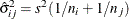 , where
  and
and  are the sizes of groups i and j, respectively, and
  is the mean square for error, with
  degrees of freedom. For weighted arithmetic means,
 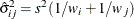 , where
  and
and  are the sums of the weights in groups i and j, respectively. Finally, for LS-means defined by the linear combinations
  and
and  of the parameter estimates,
 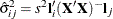 .
.
Furthermore, all of the methods are discussed in terms of significance tests of the form
where ![]() is some constant depending on the significance level. Such tests can be inverted to form confidence intervals of the form
is some constant depending on the significance level. Such tests can be inverted to form confidence intervals of the form
The simplest approach to multiple comparisons is to do a t test on every pair of means (the T option in the MEANS statement, ADJUST=T in the LSMEANS statement). For the ith and jth means, you can reject the null hypothesis that the population means are equal if
where ![]() is the significance level,
is the significance level, ![]() is the number of error degrees of freedom, and
is the number of error degrees of freedom, and ![]() is the two-tailed critical value from a Student’s t distribution. If the cell sizes are all equal to, say, n, the preceding formula can be rearranged to give
is the two-tailed critical value from a Student’s t distribution. If the cell sizes are all equal to, say, n, the preceding formula can be rearranged to give
the value of the right-hand side being Fisher’s least significant difference (LSD).
There is a problem with repeated t tests, however. Suppose there are 10 means and each t test is performed at the 0.05 level. There are ![]() pairs of means to compare, each with a 0.05 probability of a type 1 error (a false rejection of the null hypothesis). The chance of making at least one type 1 error is much higher than 0.05. It is difficult to calculate the exact
probability, but you can derive a pessimistic approximation by assuming that the comparisons are independent, giving an upper
bound to the probability of making at least one type 1 error (the experimentwise error rate) of
pairs of means to compare, each with a 0.05 probability of a type 1 error (a false rejection of the null hypothesis). The chance of making at least one type 1 error is much higher than 0.05. It is difficult to calculate the exact
probability, but you can derive a pessimistic approximation by assuming that the comparisons are independent, giving an upper
bound to the probability of making at least one type 1 error (the experimentwise error rate) of
The actual probability is somewhat less than 0.90, but as the number of means increases, the chance of making at least one type 1 error approaches 1.
If you decide to control the individual type 1 error rates for each comparison, you are controlling the individual or comparisonwise error rate. On the other hand, if you want to control the overall type 1 error rate for all the comparisons, you are controlling the experimentwise error rate. It is up to you to decide whether to control the comparisonwise error rate or the experimentwise error rate, but there are many situations in which the experimentwise error rate should be held to a small value. Statistical methods for comparing three or more means while controlling the probability of making at least one type 1 error are called multiple-comparison procedures.
It has been suggested that the experimentwise error rate can be held to the ![]() level by performing the overall ANOVA F test at the
level by performing the overall ANOVA F test at the ![]() level and making further comparisons only if the F test is significant, as in Fisher’s protected LSD. This assertion is false if there are more than three means (Einot and
Gabriel, 1975). Consider again the situation with 10 means. Suppose that one population mean differs from the others by such a sufficiently
large amount that the power (probability of correctly rejecting the null hypothesis) of the F test is near 1 but that all the other population means are equal to each other. There will be
level and making further comparisons only if the F test is significant, as in Fisher’s protected LSD. This assertion is false if there are more than three means (Einot and
Gabriel, 1975). Consider again the situation with 10 means. Suppose that one population mean differs from the others by such a sufficiently
large amount that the power (probability of correctly rejecting the null hypothesis) of the F test is near 1 but that all the other population means are equal to each other. There will be ![]() t tests of true null hypotheses, with an upper limit of 0.84 on the probability of at least one type 1 error. Thus, you must
distinguish between the experimentwise error rate under the complete null hypothesis, in which all population means are equal,
and the experimentwise error rate under a partial null hypothesis, in which some means are equal but others differ. The following
abbreviations are used in the discussion:
t tests of true null hypotheses, with an upper limit of 0.84 on the probability of at least one type 1 error. Thus, you must
distinguish between the experimentwise error rate under the complete null hypothesis, in which all population means are equal,
and the experimentwise error rate under a partial null hypothesis, in which some means are equal but others differ. The following
abbreviations are used in the discussion:
- CER
-
comparisonwise error rate
- EERC
-
experimentwise error rate under the complete null hypothesis
- MEER
-
maximum experimentwise error rate under any complete or partial null hypothesis
These error rates are associated with the different strengths of inference : individual tests control the CER; tests for inhomogeneity of means control the EERC; tests that yield confidence inequalities or confidence intervals control the MEER. A preliminary F test controls the EERC but not the MEER.
You can control the MEER at the ![]() level by setting the CER to a sufficiently small value. The Bonferroni inequality (Miller, 1981) has been widely used for this purpose. If
level by setting the CER to a sufficiently small value. The Bonferroni inequality (Miller, 1981) has been widely used for this purpose. If
where c is the total number of comparisons, then the MEER is less than ![]() . Bonferroni t tests (the BON
option in the MEANS
statement, ADJUST=BON
in the LSMEANS
statement) with
. Bonferroni t tests (the BON
option in the MEANS
statement, ADJUST=BON
in the LSMEANS
statement) with ![]() declare two means to be significantly different if
declare two means to be significantly different if
where
for comparison of k means.
Šidák (1967) has provided a tighter bound, showing that
also ensures that ![]() for any set of c comparisons. A Sidak t test (Games, 1977), provided by the SIDAK option, is thus given by
for any set of c comparisons. A Sidak t test (Games, 1977), provided by the SIDAK option, is thus given by
where
for comparison of k means.
You can use the Bonferroni additive inequality and the Sidak multiplicative inequality to control the MEER for any set of contrasts or other hypothesis tests, not just pairwise comparisons. The Bonferroni inequality can provide simultaneous inferences in any statistical application requiring tests of more than one hypothesis. Other methods discussed in this section for pairwise comparisons can also be adapted for general contrasts (Miller, 1981).
Scheffé (1953, 1959) proposes another method to control the MEER for any set of contrasts or other linear hypotheses in the analysis of linear models, including pairwise comparisons, obtained with the SCHEFFE option. Two means are declared significantly different if
where ![]() is the
is the ![]() -level critical value of an F distribution with DF numerator degrees of freedom and
-level critical value of an F distribution with DF numerator degrees of freedom and ![]() denominator degrees of freedom. The value of DF is k – 1 for the MEANS
statement, but in other statements the precise definition depends on context. For the LSMEANS
statement, DF is the rank of the contrast matrix
denominator degrees of freedom. The value of DF is k – 1 for the MEANS
statement, but in other statements the precise definition depends on context. For the LSMEANS
statement, DF is the rank of the contrast matrix ![]() for LS-means differences. In more general contexts—for example, the ESTIMATE
or LSMESTIMATE
statements in PROC GLIMMIX—DF is the rank of the contrast covariance matrix
for LS-means differences. In more general contexts—for example, the ESTIMATE
or LSMESTIMATE
statements in PROC GLIMMIX—DF is the rank of the contrast covariance matrix ![]() .
.
Scheffé’s test is compatible with the overall ANOVA F test in that Scheffé’s method never declares a contrast significant if the overall F test is nonsignificant. Most other multiple-comparison methods can find significant contrasts when the overall F test is nonsignificant and, therefore, suffer a loss of power when used with a preliminary F test.
Scheffé’s method might be more powerful than the Bonferroni or Sidak method if the number of comparisons is large relative to the number of means. For pairwise comparisons, Sidak t tests are generally more powerful.
Tukey (1952, 1953) proposes a test designed specifically for pairwise comparisons based on the studentized range, sometimes called the "honestly significant difference test," that controls the MEER when the sample sizes are equal. Tukey (1953) and Kramer (1956) independently propose a modification for unequal cell sizes. The Tukey or Tukey-Kramer method is provided by the TUKEY option in the MEANS statement and the ADJUST=TUKEY option in the LSMEANS statement. This method has fared extremely well in Monte Carlo studies (Dunnett, 1980). In addition, Hayter (1984) gives a proof that the Tukey-Kramer procedure controls the MEER for means comparisons, and Hayter (1989) describes the extent to which the Tukey-Kramer procedure has been proven to control the MEER for LS-means comparisons. The Tukey-Kramer method is more powerful than the Bonferroni, Sidak, or Scheffé method for pairwise comparisons. Two means are considered significantly different by the Tukey-Kramer criterion if
where ![]() is the
is the ![]() -level critical value of a studentized range distribution of k independent normal random variables with
-level critical value of a studentized range distribution of k independent normal random variables with ![]() degrees of freedom.
degrees of freedom.
Hochberg (1974) devised a method (the GT2 or SMM option) similar to Tukey’s, but it uses the studentized maximum modulus instead of the studentized range and employs the uncorrelated t inequality of Šidák (1967). It is proven to hold the MEER at a level not exceeding ![]() with unequal sample sizes. It is generally less powerful than the Tukey-Kramer method and always less powerful than Tukey’s
test for equal cell sizes. Two means are declared significantly different if
with unequal sample sizes. It is generally less powerful than the Tukey-Kramer method and always less powerful than Tukey’s
test for equal cell sizes. Two means are declared significantly different if
where ![]() is the
is the ![]() -level critical value of the studentized maximum modulus distribution of c independent normal random variables with
-level critical value of the studentized maximum modulus distribution of c independent normal random variables with ![]() degrees of freedom and
degrees of freedom and ![]() .
.
Gabriel (1978) proposes another method (the GABRIEL option) based on the studentized maximum modulus. This method is applicable only to arithmetic means. It rejects if
For equal cell sizes, Gabriel’s test is equivalent to Hochberg’s GT2 method. For unequal cell sizes, Gabriel’s method is more
powerful than GT2 but might become liberal with highly disparate cell sizes (see also Dunnett (1980)). Gabriel’s test is the only method for unequal sample sizes that lends itself to a graphical representation as intervals
around the means. Assuming ![]() , you can rewrite the preceding inequality as
, you can rewrite the preceding inequality as
The expression on the left does not depend on j, nor does the expression on the right depend on i. Hence, you can form what Gabriel calls an ![]() -interval around each sample mean and declare two means to be significantly different if their
-interval around each sample mean and declare two means to be significantly different if their ![]() -intervals do not overlap. See Hsu (1996, section 5.2.1.1) for a discussion of other methods of graphically representing all pairwise comparisons.
-intervals do not overlap. See Hsu (1996, section 5.2.1.1) for a discussion of other methods of graphically representing all pairwise comparisons.
One special case of means comparison is that in which the only comparisons that need to be tested are between a set of new treatments and a single control. In this case, you can achieve better power by using a method that is restricted to test only comparisons to the single control mean. Dunnett (1955) proposes a test for this situation that declares a mean significantly different from the control if
where ![]() is the control mean and
is the control mean and ![]() is the critical value of the "many-to-one t statistic" (Miller; 1981; Krishnaiah and Armitage; 1966) for k means to be compared to a control, with
is the critical value of the "many-to-one t statistic" (Miller; 1981; Krishnaiah and Armitage; 1966) for k means to be compared to a control, with ![]() error degrees of freedom and correlations
error degrees of freedom and correlations ![]() ,
, ![]() . The correlation terms arise because each of the treatment means is being compared to the same control. Dunnett’s test holds
the MEER to a level not exceeding the stated
. The correlation terms arise because each of the treatment means is being compared to the same control. Dunnett’s test holds
the MEER to a level not exceeding the stated ![]() .
.
Analysis of means (ANOM) refers to a technique for comparing group means and displaying the comparisons graphically so that you can easily see which ones are different. Means are judged as different if they are significantly different from the overall average, with significance adjusted for multiplicity. The overall average is computed as a weighted mean of the LS-means, the weights being inversely proportional to the variances. If you use the PDIFF= ANOM option in the LSMEANS statement, the procedure will display the p-values (adjusted for multiplicity, by default) for tests of the differences between each LS-mean and the average LS-mean. The ANOM procedure in SAS/QC software displays both tables and graphics for the analysis of means with a variety of response types. For one-way designs, confidence intervals for PDIFF= ANOM comparisons are equivalent to the results of PROC ANOM. The difference is that PROC GLM directly displays the confidence intervals for the differences, while the graphical output of PROC ANOM displays them as decision limits around the overall mean.
If the LS-means being compared are uncorrelated, exact adjusted p-values and critical values for confidence limits can be computed; see Nelson (1982, 1991, 1993) and Guirguis and Tobias (2004). For correlated LS-means, an approach similar to that of Hsu (1992) is employed, using a factor-analytic approximation of the correlation between the LS-means to derive approximate "effective sample sizes" for which exact critical values are computed. Note that computing the exact adjusted p-values and critical values for unbalanced designs can be computationally intensive. A simulation-based approach, as specified by the ADJUST=SIM option, while nondeterministic, might provide inferences that are accurate enough in much less time. See the section Approximate and Simulation-Based Methods for more details.
Tukey’s, Dunnett’s, and Nelson’s tests are all based on the same general quantile calculation:
where the ![]() have a joint multivariate t distribution with
have a joint multivariate t distribution with ![]() degrees of freedom and correlation matrix R. In general, evaluating
degrees of freedom and correlation matrix R. In general, evaluating ![]() requires repeated numerical calculation of an
requires repeated numerical calculation of an ![]() -fold integral. This is usually intractable, but the problem reduces to a feasible 2-fold integral when R has a certain symmetry in the case of Tukey’s test, and a factor analytic structure (Hsu; 1992) in the case of Dunnett’s and Nelson’s tests. The R matrix has the required symmetry for exact computation of Tukey’s test in the following two cases:
-fold integral. This is usually intractable, but the problem reduces to a feasible 2-fold integral when R has a certain symmetry in the case of Tukey’s test, and a factor analytic structure (Hsu; 1992) in the case of Dunnett’s and Nelson’s tests. The R matrix has the required symmetry for exact computation of Tukey’s test in the following two cases:
-
The
 s are studentized differences between
  pairs of k uncorrelated means with equal variances—that is, equal sample sizes.
-
The
s are studentized differences between pairs of k LS-means from a variance-balanced design (for example, a balanced incomplete block design).
See Hsu (1992, 1996) for more information. The R matrix has the factor analytic structure for exact computation of Dunnett’s and Nelson’s tests in the following two cases:
-
if the
s are studentized differences between k – 1 means and a control mean, all uncorrelated. (Dunnett’s one-sided methods depend on a similar probability calculation,
without the absolute values.) Note that it is not required that the variances of the means (that is, the sample sizes) be
equal.
-
if the
s are studentized differences between k – 1 LS-means and a control LS-mean from either a variance-balanced design, or a design in which the other factors are orthogonal to the treatment factor (for example, a randomized block design with proportional cell frequencies)
However, other important situations that do not result in a correlation matrix R that has the structure for exact computation are the following:
-
all pairwise differences with unequal sample sizes
-
differences between LS-means in many unbalanced designs
In these situations, exact calculation of ![]() is intractable in general. Most of the preceding methods can be viewed as using various approximations for
is intractable in general. Most of the preceding methods can be viewed as using various approximations for ![]() . When the sample sizes are unequal, the Tukey-Kramer test is equivalent to another approximation. For comparisons with a
control when the correlation R does not have a factor analytic structure, Hsu (1992) suggests approximating R with a matrix
. When the sample sizes are unequal, the Tukey-Kramer test is equivalent to another approximation. For comparisons with a
control when the correlation R does not have a factor analytic structure, Hsu (1992) suggests approximating R with a matrix ![]() that does have such a structure and correspondingly approximating
that does have such a structure and correspondingly approximating ![]() with
with ![]() . When you request Dunnett’s or Nelson’s test for LS-means (the PDIFF=CONTROL and ADJUST=DUNNETT
options or the PDIFF=
ANOM and ADJUST=NELSON
options, respectively), the GLM procedure automatically uses Hsu’s approximation when appropriate.
. When you request Dunnett’s or Nelson’s test for LS-means (the PDIFF=CONTROL and ADJUST=DUNNETT
options or the PDIFF=
ANOM and ADJUST=NELSON
options, respectively), the GLM procedure automatically uses Hsu’s approximation when appropriate.
Finally, Edwards and Berry (1987) suggest calculating ![]() by simulation. Multivariate t vectors are sampled from a distribution with the appropriate
by simulation. Multivariate t vectors are sampled from a distribution with the appropriate ![]() and R parameters, and Edwards and Berry (1987) suggest estimating
and R parameters, and Edwards and Berry (1987) suggest estimating ![]() by
by ![]() , the
, the ![]() percentile of the observed values of
percentile of the observed values of ![]() . Sufficient samples are generated for the true
. Sufficient samples are generated for the true ![]() to be within a certain accuracy radius
to be within a certain accuracy radius ![]() of
of ![]() with accuracy confidence
with accuracy confidence ![]() . You can approximate
. You can approximate ![]() by simulation for comparisons between LS-means by specifying ADJUST=SIM
(with any PDIFF=
type). By default,
by simulation for comparisons between LS-means by specifying ADJUST=SIM
(with any PDIFF=
type). By default, ![]() and
and ![]() , so that the tail area of
, so that the tail area of ![]() is within 0.005 of
is within 0.005 of ![]() with 99% confidence. You can use the ACC= and EPS= options with ADJUST=SIM
to reset
with 99% confidence. You can use the ACC= and EPS= options with ADJUST=SIM
to reset ![]() and
and ![]() , or you can use the NSAMP= option to set the sample size directly. You can also control the random number sequence with the
SEED= option.
, or you can use the NSAMP= option to set the sample size directly. You can also control the random number sequence with the
SEED= option.
Hsu and Nelson (1998) suggest a more accurate simulation method for estimating ![]() , using a control variate adjustment technique. The same independent, standardized normal variates that are used to generate
multivariate t vectors from a distribution with the appropriate
, using a control variate adjustment technique. The same independent, standardized normal variates that are used to generate
multivariate t vectors from a distribution with the appropriate ![]() and R parameters are also used to generate multivariate t vectors from a distribution for which the exact value of
and R parameters are also used to generate multivariate t vectors from a distribution for which the exact value of ![]() is known.
is known. ![]() for the second sample is used as a control variate for adjusting the quantile estimate based on the first sample; see Hsu
and Nelson (1998) for more details. The control variate adjustment has the drawback that it takes somewhat longer than the crude technique
of Edwards and Berry (1987), but it typically yields an estimate that is many times more accurate. In most cases, if you are using ADJUST=SIM
, then you should specify ADJUST=SIM(CVADJUST). You can also specify ADJUST=SIM(CVADJUST REPORT) to display a summary of the
simulation that includes, among other things, the actual accuracy radius
for the second sample is used as a control variate for adjusting the quantile estimate based on the first sample; see Hsu
and Nelson (1998) for more details. The control variate adjustment has the drawback that it takes somewhat longer than the crude technique
of Edwards and Berry (1987), but it typically yields an estimate that is many times more accurate. In most cases, if you are using ADJUST=SIM
, then you should specify ADJUST=SIM(CVADJUST). You can also specify ADJUST=SIM(CVADJUST REPORT) to display a summary of the
simulation that includes, among other things, the actual accuracy radius ![]() , which should be substantially smaller than the target accuracy radius (0.005 by default).
, which should be substantially smaller than the target accuracy radius (0.005 by default).
You can use all of the methods discussed so far to obtain simultaneous confidence intervals (Miller, 1981). By sacrificing the facility for simultaneous estimation, you can obtain simultaneous tests with greater power by using multiple-stage tests (MSTs). MSTs come in both step-up and step-down varieties (Welsch, 1977). The step-down methods, which have been more widely used, are available in SAS/STAT software.
Step-down MSTs first test the homogeneity of all the means at a level ![]() . If the test results in a rejection, then each subset of k – 1 means is tested at level
. If the test results in a rejection, then each subset of k – 1 means is tested at level ![]() ; otherwise, the procedure stops. In general, if the hypothesis of homogeneity of a set of p means is rejected at the
; otherwise, the procedure stops. In general, if the hypothesis of homogeneity of a set of p means is rejected at the ![]() level, then each subset of
level, then each subset of ![]() means is tested at the
means is tested at the ![]() level; otherwise, the set of p means is considered not to differ significantly and none of its subsets are tested. The many varieties of MSTs that have
been proposed differ in the levels
level; otherwise, the set of p means is considered not to differ significantly and none of its subsets are tested. The many varieties of MSTs that have
been proposed differ in the levels ![]() and the statistics on which the subset tests are based. Clearly, the EERC of a step-down MST is not greater than
and the statistics on which the subset tests are based. Clearly, the EERC of a step-down MST is not greater than ![]() , and the CER is not greater than
, and the CER is not greater than ![]() , but the MEER is a complicated function of
, but the MEER is a complicated function of ![]() ,
, ![]() .
.
With unequal cell sizes, PROC GLM uses the harmonic mean of the cell sizes as the common sample size. However, since the resulting operating characteristics can be undesirable, MSTs are recommended only for the balanced case. When the sample sizes are equal, using the range statistic enables you to arrange the means in ascending or descending order and test only contiguous subsets. But if you specify the F statistic, this shortcut cannot be taken. For this reason, only range-based MSTs are implemented. It is common practice to report the results of an MST by writing the means in such an order and drawing lines parallel to the list of means spanning the homogeneous subsets. This form of presentation is also convenient for pairwise comparisons with equal cell sizes.
The best-known MSTs are the Duncan (the DUNCAN option) and Student-Newman-Keuls (the SNK option) methods (Miller, 1981). Both use the studentized range statistic and, hence, are called multiple range tests. Duncan’s method is often called the "new" multiple range test despite the fact that it is one of the oldest MSTs in current use.
The Duncan and SNK methods differ in the ![]() values used. For Duncan’s method, they are
values used. For Duncan’s method, they are
whereas the SNK method uses
Duncan’s method controls the CER at the ![]() level. Its operating characteristics appear similar to those of Fisher’s unprotected LSD or repeated t tests at level
level. Its operating characteristics appear similar to those of Fisher’s unprotected LSD or repeated t tests at level ![]() (Petrinovich and Hardyck, 1969). Since repeated t tests are easier to compute, easier to explain, and applicable to unequal sample sizes, Duncan’s method is not recommended.
Several published studies (for example, Carmer and Swanson (1973)) have claimed that Duncan’s method is superior to Tukey’s because of greater power without considering that the greater
power of Duncan’s method is due to its higher type 1 error rate (Einot and Gabriel, 1975).
(Petrinovich and Hardyck, 1969). Since repeated t tests are easier to compute, easier to explain, and applicable to unequal sample sizes, Duncan’s method is not recommended.
Several published studies (for example, Carmer and Swanson (1973)) have claimed that Duncan’s method is superior to Tukey’s because of greater power without considering that the greater
power of Duncan’s method is due to its higher type 1 error rate (Einot and Gabriel, 1975).
The SNK method holds the EERC to the ![]() level but does not control the MEER (Einot and Gabriel, 1975). Consider ten population means that occur in five pairs such that means within a pair are equal, but there are large differences
between pairs. If you make the usual sampling assumptions and also assume that the sample sizes are very large, all subset
homogeneity hypotheses for three or more means are rejected. The SNK method then comes down to five independent tests, one
for each pair, each at the
level but does not control the MEER (Einot and Gabriel, 1975). Consider ten population means that occur in five pairs such that means within a pair are equal, but there are large differences
between pairs. If you make the usual sampling assumptions and also assume that the sample sizes are very large, all subset
homogeneity hypotheses for three or more means are rejected. The SNK method then comes down to five independent tests, one
for each pair, each at the ![]() level. Letting
level. Letting ![]() be 0.05, the probability of at least one false rejection is
be 0.05, the probability of at least one false rejection is
As the number of means increases, the MEER approaches 1. Therefore, the SNK method cannot be recommended.
A variety of MSTs that control the MEER have been proposed, but these methods are not as well known as those of Duncan and SNK. One approach (Ryan, 1959, 1960; Einot and Gabriel, 1975; Welsch, 1977) sets
You can use range statistics, leading to what is called the REGWQ method, after the authors’ initials. If you assume that the sample means have been arranged in descending order from ![]() through
through ![]() , the homogeneity of means
, the homogeneity of means ![]() , is rejected by REGWQ if
, is rejected by REGWQ if
where ![]() and the summations are over
and the summations are over ![]() (Einot and Gabriel, 1975). To ensure that the MEER is controlled, the current implementation checks whether
(Einot and Gabriel, 1975). To ensure that the MEER is controlled, the current implementation checks whether ![]() is monotonically increasing in p. If not, then a set of critical values that are increasing in p is substituted instead.
is monotonically increasing in p. If not, then a set of critical values that are increasing in p is substituted instead.
REGWQ appears to be the most powerful step-down MST in the current literature (for example, Ramsey; 1978). Use of a preliminary F test decreases the power of all the other multiple-comparison methods discussed previously except for Scheffé’s test.
Waller and Duncan (1969) and Duncan (1975) take an approach to multiple comparisons that differs from all the methods previously discussed in minimizing the Bayes
risk under additive loss rather than controlling type 1 error rates. For each pair of population means ![]() and
and ![]() , null
, null ![]() and alternative
and alternative ![]() hypotheses are defined:
hypotheses are defined:
![\begin{eqnarray*} H_0^{ij}\colon & & \mu _ i - \mu _ j \leq 0 \\[0.05in] H_ a^{ij}\colon & & \mu _ i - \mu _ j > 0 \end{eqnarray*}](images/statug_glm0249.png)
For any i, j pair, let ![]() indicate a decision in favor of
indicate a decision in favor of ![]() and
and ![]() indicate a decision in favor of
indicate a decision in favor of ![]() , and let
, and let ![]() . The loss function for the decision on the i, j pair is
. The loss function for the decision on the i, j pair is
![\begin{eqnarray*} L(d_0~ |~ \delta ) & = & \left\{ \begin{array}{lcl} 0 & & \mbox{if~ } \delta \leq 0 \\[0.05in] \delta & & \mbox{if~ } \delta > 0 \\ \end{array}\right. \\[0.10in] L(d_ a~ |~ \delta ) & = & \left\{ \begin{array}{lcl} -k \delta & & \mbox{if~ } \delta \leq 0 \\[0.05in] 0 & & \mbox{if~ } \delta > 0 \\ \end{array}\right. \end{eqnarray*}](images/statug_glm0255.png)
where k represents a constant that you specify rather than the number of means. The loss for the joint decision involving all pairs of means is the sum of the losses for each individual decision. The population means are assumed to have a normal prior distribution with unknown variance, the logarithm of the variance of the means having a uniform prior distribution. For the i, j pair, the null hypothesis is rejected if
where ![]() is the Bayesian t value (Waller and Kemp, 1976) depending on k, the F statistic for the one-way ANOVA, and the degrees of freedom for F. The value of
is the Bayesian t value (Waller and Kemp, 1976) depending on k, the F statistic for the one-way ANOVA, and the degrees of freedom for F. The value of ![]() is a decreasing function of F, so the Waller-Duncan test (specified by the WALLER
option) becomes more liberal as F increases.
is a decreasing function of F, so the Waller-Duncan test (specified by the WALLER
option) becomes more liberal as F increases.
In summary, if you are interested in several individual comparisons and are not concerned about the effects of multiple inferences, you can use repeated t tests or Fisher’s unprotected LSD. If you are interested in all pairwise comparisons or all comparisons with a control, you should use Tukey’s or Dunnett’s test, respectively, in order to make the strongest possible inferences. If you have weaker inferential requirements and, in particular, if you do not want confidence intervals for the mean differences, you should use the REGWQ method. Finally, if you agree with the Bayesian approach and Waller and Duncan’s assumptions, you should use the Waller-Duncan test.
When you interpret multiple comparisons, remember that failure to reject the hypothesis that two or more means are equal should not lead you to conclude that the population means are, in fact, equal. Failure to reject the null hypothesis implies only that the difference between population means, if any, is not large enough to be detected with the given sample size. A related point is that nonsignificance is nontransitive: that is, given three sample means, the largest and smallest might be significantly different from each other, while neither is significantly different from the middle one. Nontransitive results of this type occur frequently in multiple comparisons.
Multiple comparisons can also lead to counterintuitive results when the cell sizes are unequal. Consider four cells labeled A, B, C, and D, with sample means in the order A>B>C>D. If A and D each have two observations, and B and C each have 10,000 observations, then the difference between B and C might be significant, while the difference between A and D is not.
[29] The Duncan-Waller method does not fit into the preceding scheme, since it is based on the Bayes risk rather than any particular error rate.