The LIFEREG Procedure
- Overview
-
Getting Started

-
Syntax
-
DetailsMissing ValuesModel SpecificationComputational MethodSupported DistributionsPredicted ValuesConfidence IntervalsFit StatisticsProbability PlottingINEST= Data SetOUTEST= Data SetXDATA= Data SetComputational ResourcesBayesian AnalysisDisplayed Output for Classical AnalysisDisplayed Output for Bayesian AnalysisODS Table NamesODS Graphics
-
ExamplesMotorette FailureComputing Predicted Values for a Tobit ModelOvercoming Convergence Problems by Specifying Initial ValuesAnalysis of Arbitrarily Censored Data with Interaction EffectsProbability Plotting—Right CensoringProbability Plotting—Arbitrary CensoringBayesian Analysis of Clinical Trial DataModel Postfitting Analysis
- References
Nelson (1982) describes a study of the lifetimes of locomotive engine fans. This example shows how to use PROC LIFEREG to carry out a Bayesian analysis of the engine fan data. In this example, a lognormal distribution is used to model the engine lifetimes, but other survival time distributions, such as the Weibull, can also be used.
The following SAS statements create the SAS data set Fan. This data set contains a censoring indicator variable and right-censored survival times for the 70 locomotive engine fans
in the study.
data Fan;
   input Lifetime Censor@@;
   datalines;
 450 0    460 1   1150 0   1150 0   1560 1
1600 0   1660 1   1850 1   1850 1   1850 1
1850 1   1850 1   2030 1   2030 1   2030 1
2070 0   2070 0   2080 0   2200 1   3000 1
3000 1   3000 1   3000 1   3100 0   3200 1
3450 0   3750 1   3750 1   4150 1   4150 1
4150 1   4150 1   4300 1   4300 1   4300 1
4300 1   4600 0   4850 1   4850 1   4850 1
4850 1   5000 1   5000 1   5000 1   6100 1
6100 0   6100 1   6100 1   6300 1   6450 1
6450 1   6700 1   7450 1   7800 1   7800 1
8100 1   8100 1   8200 1   8500 1   8500 1
8500 1   8750 1   8750 0   8750 1   9400 1
9900 1  10100 1  10100 1  10100 1  11500 1
;
Some of the fans had not failed at the time the data were collected, and the unfailed units have right-censored lifetimes.
The variable Lifetime represents either a failure time or a censoring time. The variable Censor is equal to 0 if the value of Lifetime is a failure time, and it is equal to 1 if the value is a censoring time.
The following SAS statements specify a Bayesian analysis that uses a lognormal model for the engine lifetimes. There are no
covariates, so the model is an intercept-only model. The OUTPOST= option saves the samples from the posterior distribution
in the SAS data set Post for further processing.
ods graphics on;
proc lifereg data=Fan;
   model Lifetime*Censor( 1 )= / dist=lognormal;
   bayes seed=1  outpost=Post;
run;
ods graphics off;
The SEED= option is specified to maintain reproducibility; no other options are specified in the BAYES statement. By default,
a uniform prior distribution is assumed for the intercept coefficient. The uniform prior is a flat prior on the real line
with a distribution that reflects ignorance of the location of the parameter, placing equal probability on all possible values
the regression coefficient can take. Using the uniform prior in the following example, you would expect the Bayesian estimates
to resemble the classical results of maximizing the likelihood. If you can elicit an informative prior on the regression coefficients,
you should use the COEFFPRIOR= option to specify it. A default noninformative gamma prior is used for the lognormal scale
parameter ![]() .
.
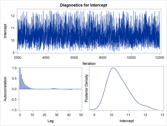
You should make sure that the posterior distribution samples have achieved convergence before using them for Bayesian inference. If you do not specify additional options, PROC LIFEREG produces by default three convergence diagnostics: autocorrelations of the posterior sample, effective sample size, and the Geweke statistic. See the section Assessing Markov Chain Convergence in Chapter 7: Introduction to Bayesian Analysis Procedures, for information about assessing the convergence of the chain of posterior samples. Trace plots, posterior density plots, and autocorrelation function plots that are created using ODS Graphics are also provided for each parameter. See the section Visual Analysis via Trace Plots in Chapter 7: Introduction to Bayesian Analysis Procedures, for help in interpreting these plots.
The “Analysis of Maximum Likelihood Parameter Estimates” table in Figure 55.6 summarizes maximum likelihood estimates of the lognormal intercept and scale parameters.
Figure 55.6: Maximum Likelihood Estimates from the LIFEREG Procedure
| Analysis of Maximum Likelihood Parameter Estimates | |||||
|---|---|---|---|---|---|
| Parameter | DF | Estimate | Standard Error | 95% Confidence Limits | |
| Intercept | 1 | 10.1432 | 0.5211 | 9.1219 | 11.1646 |
| Scale | 1 | 1.6796 | 0.3893 | 1.0664 | 2.6453 |
Since no prior distribution for the intercept was specified, the default uniform improper distribution shown in the “Uniform Prior for Regression Coefficients” table in Figure 55.7 is used.
Noninformative prior distributions are appropriate if you have no prior knowledge of the likely range of values of the parameters, and if you want to make probability statements about the parameters or functions of the parameters. Refer, for example, to Ibrahim, Chen, and Sinha (2001) for more information about choosing prior distributions.
The default noninformative gamma prior distribution for the lognormal scale parameter is shown in the “Independent Prior Distributions for Model Parameters” table in Figure 55.7.
Figure 55.7: Noninformative Prior Distributions
| Uniform Prior for Regression Coefficients |
|
|---|---|
| Parameter | Prior |
| Intercept | Constant |
| Independent Prior Distributions for Model Parameters | |||||
|---|---|---|---|---|---|
| Parameter | Prior Distribution | Hyperparameters | |||
| Scale | Gamma | Shape | 0.001 | Inverse Scale | 0.001 |
By default, posterior mode estimates of the model parameters are used as the starting value for the simulation. These are listed in the “Initial Values of the Chain” table in Figure 55.8.
Figure 55.8: Markov Chain Initial Values
| Initial Values of the Chain | |||
|---|---|---|---|
| Chain | Seed | Intercept | Scale |
| 1 | 1 | 10.0501 | 1.59544 |
Summary statistics for the posterior sample are displayed in the “Fit Statistics,” “Descriptive Statistics for the Posterior Sample,” “Interval Statistics for the Posterior Sample,” and “Posterior Correlation Matrix” tables in Figure 55.9. Since noninformative prior distributions were used, these results are consistent with the maximum likelihood estimates shown in Figure 55.6.
Figure 55.9: Posterior Sample Summary Statistics
| Fit Statistics | |
|---|---|
| DIC (smaller is better) | 87.245 |
| pD (effective number of parameters) | 1.823 |
| Posterior Summaries | ||||||
|---|---|---|---|---|---|---|
| Parameter | N | Mean | Standard Deviation |
Percentiles | ||
| 25% | 50% | 75% | ||||
| Intercept | 10000 | 10.4196 | 0.6172 | 9.9670 | 10.3259 | 10.7959 |
| Scale | 10000 | 1.9196 | 0.4809 | 1.5675 | 1.8476 | 2.1931 |
| Posterior Intervals | |||||
|---|---|---|---|---|---|
| Parameter | Alpha | Equal-Tail Interval | HPD Interval | ||
| Intercept | 0.050 | 9.4477 | 11.8994 | 9.3216 | 11.6752 |
| Scale | 0.050 | 1.1906 | 3.0570 | 1.1104 | 2.8834 |
| Posterior Correlation Matrix | ||
|---|---|---|
| Parameter | Intercept | Scale |
| Intercept | 1.0000 | 0.8297 |
| Scale | 0.8297 | 1.0000 |
By default, PROC LIFEREG computes three convergence diagnostics: the lag1, lag5, lag10, and lag50 autocorrelations; the Geweke
diagnostic; and the effective sample size. These are displayed in Figure 55.10. There is no indication that the Markov chain has not converged. See the section Assessing Markov Chain Convergence in Chapter 7: Introduction to Bayesian Analysis Procedures, for more information about convergence diagnostics and their interpretation.
Figure 55.10: Posterior Sample Summary Statistics
| Posterior Autocorrelations | ||||
|---|---|---|---|---|
| Parameter | Lag 1 | Lag 5 | Lag 10 | Lag 50 |
| Intercept | 0.6973 | 0.1765 | 0.0190 | -0.0017 |
| Scale | 0.6955 | 0.1713 | 0.0172 | -0.0002 |
| Geweke Diagnostics | ||
|---|---|---|
| Parameter | z | Pr > |z| |
| Intercept | -0.9183 | 0.3585 |
| Scale | -0.9233 | 0.3559 |
| Effective Sample Sizes | |||
|---|---|---|---|
| Parameter | ESS | Autocorrelation Time |
Efficiency |
| Intercept | 1772.8 | 5.6408 | 0.1773 |
| Scale | 1805.0 | 5.5400 | 0.1805 |
Summary statistics of the posterior distribution samples are produced by default. However, these statistics might not be sufficient
for carrying out your Bayesian inference. The samples from the posterior distribution saved in the SAS data set Post created with the OUTPOST= option can be used for further analysis. Trace, autocorrelation, and density plots for the three
model parameters shown in Figure 55.11 and Figure 55.12 are useful in diagnosing whether the Markov chain of posterior samples has converged. These plots show no evidence that the
chain has not converged. See the section Visual Analysis via Trace Plots in Chapter 7: Introduction to Bayesian Analysis Procedures, for more information about interpreting these types of diagnostic plots.

The fraction failing in the first 8000 hours of operation might be a quantity of interest. This kind of information could
be useful, for example, in determining whether to improve the reliability of the engine components due to warranty considerations.
The following SAS statements compute the mean and percentiles of the distribution of the fraction failing in the first 8000
hours from the posterior sample data set Post:
data Prob;
   set Post;
   Frac = ProbNorm(( log(8000) - Intercept ) / Scale );
   label Frac= 'Fraction Failing in 8000 Hours';
run;

proc means data = Prob(keep=Frac) n mean p10 p25 p50 p75 p90;
run;
The mean fraction of failures in the first 8000 hours, shown in Figure 55.13, is about 0.24, which could be used in further analysis of warranty costs. The 10th percentile is about 0.16 and the 90th percentile is about 0.32, which gives an assessment of the probable range of the fraction failing in the first 8000 hours.
Figure 55.13: Fraction Failing in 8000 Hours
| Analysis Variable : Frac Fraction Failing in 8000 Hours | ||||||
|---|---|---|---|---|---|---|
| N | Mean | 10th Pctl | 25th Pctl | 50th Pctl | 75th Pctl | 90th Pctl |
| 10000 | 0.2381467 | 0.1628591 | 0.1953691 | 0.2336756 | 0.2766051 | 0.3190883 |