The PHREG Procedure
- Overview
-
Getting Started

-
SyntaxPROC PHREG StatementASSESS StatementBASELINE StatementBAYES StatementBY StatementCLASS StatementCONTRAST StatementEFFECT StatementESTIMATE StatementFREQ StatementHAZARDRATIO StatementID StatementLSMEANS StatementLSMESTIMATE StatementMODEL StatementOUTPUT StatementProgramming StatementsRANDOM StatementSTRATA StatementSLICE StatementSTORE StatementTEST StatementWEIGHT Statement
-
DetailsFailure Time DistributionTime and CLASS Variables UsagePartial Likelihood Function for the Cox ModelCounting Process Style of InputLeft-Truncation of Failure TimesThe Multiplicative Hazards ModelThe Frailty ModelHazard RatiosProportional Rates/Means Models for Recurrent EventsNewton-Raphson MethodFirth’s Modification for Maximum Likelihood EstimationRobust Sandwich Variance EstimateTesting the Global Null HypothesisType 3 TestsConfidence Limits for a Hazard RatioUsing the TEST Statement to Test Linear HypothesesAnalysis of Multivariate Failure Time DataModel Fit StatisticsResidualsDiagnostics Based on Weighted ResidualsInfluence of Observations on Overall Fit of the ModelSurvivor Function EstimatorsEffect Selection MethodsAssessment of the Proportional Hazards ModelThe Penalized Partial Likelihood Approach for Fitting Frailty ModelsSpecifics for Bayesian AnalysisComputational ResourcesInput and Output Data SetsDisplayed OutputODS Table NamesODS Graphics
-
ExamplesStepwise RegressionBest Subset SelectionModeling with Categorical PredictorsFirth’s Correction for Monotone LikelihoodConditional Logistic Regression for m:n MatchingModel Using Time-Dependent Explanatory VariablesTime-Dependent Repeated Measurements of a CovariateSurvival CurvesAnalysis of ResidualsAnalysis of Recurrent Events DataAnalysis of Clustered DataModel Assessment Using Cumulative Sums of Martingale ResidualsBayesian Analysis of the Cox ModelBayesian Analysis of Piecewise Exponential Model
- References
PROC PHREG uses the partial likelihood of the Cox model as the likelihood and generates a chain of posterior distribution samples by the Gibbs Sampler. Summary statistics, convergence diagnostics, and diagnostic plots are provided for each parameter. The following statements generate Figure 67.4–Figure 67.10:
ods graphics on;
proc phreg data=Rats;
   model Days*Status(0)=Group;
   bayes seed=1 outpost=Post;
run;
ods graphics off;
The BAYES statement invokes the Bayesian analysis. The SEED= option is specified to maintain reproducibility; the OUTPOST=
option saves the posterior distribution samples in a SAS data set for post-processing; no other options are specified in the
BAYES statement. By default, a uniform prior distribution is assumed on the regression coefficient Group. The uniform prior is a flat prior on the real line with a distribution that reflects ignorance of the location of the parameter,
placing equal probability on all possible values the regression coefficient can take. Using the uniform prior in the following
example, you would expect the Bayesian estimates to resemble the classical results of maximizing the likelihood. If you can
elicit an informative prior on the regression coefficients, you should use the COEFFPRIOR= option to specify it.
You should make sure that the posterior distribution samples have achieved convergence before using them for Bayesian inference. PROC PHREG produces three convergence diagnostics by default. If ODS Graphics is enabled before calling PROC PHREG as in the preceding program, diagnostics plots are also displayed.
The results of this analysis are shown in the following figures.
The “Model Information” table in Figure 67.4 summarizes information about the model you fit and the size of the simulation.
Figure 67.4: Model Information
| Model Information | ||
|---|---|---|
| Data Set | WORK.RATS | |
| Dependent Variable | Days | Days from Exposure to Death |
| Censoring Variable | Status | |
| Censoring Value(s) | 0 | |
| Model | Cox | |
| Ties Handling | BRESLOW | |
| Sampling Algorithm | ARMS | |
| Burn-In Size | 2000 | |
| MC Sample Size | 10000 | |
| Thinning | 1 | |
PROC PHREG first fits the Cox model by maximizing the partial likelihood. The only parameter in the model is the regression
coefficient of Group. The maximum likelihood estimate (MLE) of the parameter and its 95% confidence interval are shown in Figure 67.5.
Figure 67.5: Classical Parameter Estimates
| Maximum Likelihood Estimates | |||||
|---|---|---|---|---|---|
| Parameter | DF | Estimate | Standard Error |
95% Confidence Limits | |
| Group | 1 | -0.5959 | 0.3484 | -1.2788 | 0.0870 |
Since no prior is specified for the regression coefficient, the default uniform prior is used. This information is displayed in the “Uniform Prior for Regression Coefficients” table in Figure 67.6.
Figure 67.6: Coefficient Prior
| Uniform Prior for Regression Coefficients |
|
|---|---|
| Parameter | Prior |
| Group | Constant |
The “Fit Statistics” table in Figure 67.7 lists information about the fitted model. The table displays the DIC (deviance information criterion) and pD (effective number of parameters). See the section Fit Statistics for details.
Figure 67.7: Fit Statistics
| Fit Statistics | |
|---|---|
| DIC (smaller is better) | 203.444 |
| pD (Effective Number of Parameters) | 1.003 |
Summary statistics of the posterior samples are displayed in the “Posterior Summaries” table and “Posterior Intervals” table as shown in Figure 67.8. Note that the mean and standard deviation of the posterior samples are comparable to the MLE and its standard error, respectively, due to the use of the uniform prior.
Figure 67.8: Summary Statistics
| Posterior Summaries | ||||||
|---|---|---|---|---|---|---|
| Parameter | N | Mean | Standard Deviation |
Percentiles | ||
| 25% | 50% | 75% | ||||
| Group | 10000 | -0.5998 | 0.3511 | -0.8326 | -0.5957 | -0.3670 |
| Posterior Intervals | |||||
|---|---|---|---|---|---|
| Parameter | Alpha | Equal-Tail Interval | HPD Interval | ||
| Group | 0.050 | -1.3042 | 0.0721 | -1.2984 | 0.0756 |
PROC PHREG provides diagnostics to assess the convergence of the generated Markov chain. Figure 67.9 shows three of these diagnostics: the lag1, lag5, lag10, and lag50 autocorrelations; the Geweke diagnostic; and the effective sample size. There is no indication that the Markov chain has not reached convergence. See the section Statistical Diagnostic Tests for information about interpreting these diagnostics.
Figure 67.9: Convergence Diagnostics
| Posterior Autocorrelations | ||||
|---|---|---|---|---|
| Parameter | Lag 1 | Lag 5 | Lag 10 | Lag 50 |
| Group | -0.0079 | 0.0091 | -0.0161 | 0.0101 |
| Geweke Diagnostics | ||
|---|---|---|
| Parameter | z | Pr > |z| |
| Group | 0.0149 | 0.9881 |
| Effective Sample Sizes | |||
|---|---|---|---|
| Parameter | ESS | Autocorrelation Time |
Efficiency |
| Group | 10000.0 | 1.0000 | 1.0000 |
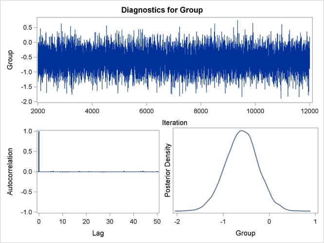
You can also assess the convergence of the generated Markov chain by examining the trace plot, the autocorrelation function
plot, and the posterior density plot. Figure 67.10 displays a panel of these three plots for the parameter Group. This graphical display is automatically produced when ODS Graphics is enabled. Note that the trace of the samples centers
on –0.6 with only small fluctuations, the autocorrelations are quite small, and the posterior density appears bell-shaped—all
exemplifying the behavior of a converged Markov chain.
The proportional hazards model for comparing the two pretreatment groups is
The probability that the hazard of Group=0 is greater than that of Group=1 is
This probability can be enumerated from the posterior distribution samples by computing the fraction of samples with a coefficient less than 0. The following DATA step and PROC MEANS perform this calculation:
data New;
   set Post;
   Indicator=(Group < 0);
   label Indicator='Group < 0';
run;
proc means data=New(keep=Indicator) n mean;
run;
Figure 67.11: Prob(Hazard(Group=0) > Hazard(Group=1))
| Analysis Variable : Indicator Group < 0 |
|
|---|---|
| N | Mean |
| 10000 | 0.9581000 |
The PROC MEANS results are displayed in Figure 67.11. There is a 95.8% chance that the hazard rate of Group=0 is greater than that of Group=1. The result is consistent with the fact that the average survival time of Group=0 is less than that of Group=1.