The SEQDESIGN Procedure
-
Overview

- Getting Started
-
Syntax
-
DetailsFixed-Sample Clinical TrialsOne-Sided Fixed-Sample Tests in Clinical TrialsTwo-Sided Fixed-Sample Tests in Clinical TrialsGroup Sequential MethodsStatistical Assumptions for Group Sequential DesignsBoundary ScalesBoundary VariablesType I and Type II ErrorsUnified Family MethodsHaybittle-Peto MethodWhitehead MethodsError Spending MethodsAcceptance (beta) BoundaryBoundary Adjustments for Overlapping Lower and Upper beta BoundariesSpecified and Derived ParametersApplicable Boundary KeysSample Size ComputationApplicable One-Sample Tests and Sample Size ComputationApplicable Two-Sample Tests and Sample Size ComputationApplicable Regression Parameter Tests and Sample Size ComputationAspects of Group Sequential DesignsSummary of Methods in Group Sequential DesignsTable OutputODS Table NamesGraphics OutputODS Graphics
-
ExamplesCreating Fixed-Sample DesignsCreating a One-Sided O’Brien-Fleming DesignCreating Two-Sided Pocock and O’Brien-Fleming DesignsGenerating Graphics Display for Sequential DesignsCreating Designs Using Haybittle-Peto MethodsCreating Designs with Various Stopping CriteriaCreating Whitehead’s Triangular DesignsCreating a One-Sided Error Spending DesignCreating Designs with Various Number of StagesCreating Two-Sided Error Spending Designs with and without Overlapping Lower and Upper beta BoundariesCreating a Two-Sided Asymmetric Error Spending Design with Early Stopping to Reject H0Creating a Two-Sided Asymmetric Error Spending Design with Early Stopping to Reject or Accept H0Creating a Design with a Nonbinding Beta BoundaryComputing Sample Size for Survival Data
- References
Example 83.7 Creating Whitehead’s Triangular Designs
This example requests three 4-stage Whitehead’s triangular designs for normally distributed statistics. Each design has a
one-sided alternative hypothesis with early stopping to reject or accept the null hypothesis ![]() . Note that Whitehead’s triangular designs are different from unified family triangular designs.
. Note that Whitehead’s triangular designs are different from unified family triangular designs.
Suppose that a clinic is conducting a study of the effect of a new cancer treatment. The study consists of exposing mice to a carcinogen and randomly assigning them to either the control group or the treatment group. The event of interest is death from cancer induced by the carcinogen, and the response is the time from randomization to death.
Following the derivations in the section Test for Two Survival Distributions with a Log-Rank Test, the hypothesis ![]() with an alternative hypothesis
with an alternative hypothesis ![]() is used, where
is used, where ![]() is the hazard ratio between the treatment group and the control group.
is the hazard ratio between the treatment group and the control group.
Also suppose that from past experience, the median survival time for the control group is ![]() weeks, and the study wants to detect a
weeks, and the study wants to detect a ![]() weeks’ median survival time with a 80% power in the trial. Assuming exponential survival functions for the two groups, the
hazard rates can be computed from
weeks’ median survival time with a 80% power in the trial. Assuming exponential survival functions for the two groups, the
hazard rates can be computed from
|
|
where ![]() .
.
Thus, with ![]() and
and ![]() , the hazard ratio
, the hazard ratio ![]() , and the alternative reference is
, and the alternative reference is
|
|
The following statements invoke the SEQDESIGN procedure and specify three Whitehead’s triangular designs:
ods graphics on;
proc seqdesign altref=0.693147
               bscale=score
               plots=combinedboundary
               ;
   BoundaryKeyNone:  design nstages=4
                            method=whitehead
                            boundarykey=none
                            alt=upper   stop=both
                            alpha=0.05  beta=0.20
                            ;
   BoundaryKeyAlpha: design nstages=4
                            method=whitehead
                            boundarykey=alpha
                            alt=upper   stop=both
                            alpha=0.05  beta=0.20
                            ;

   BoundaryKeyBeta:  design nstages=4
                            method=whitehead
                            boundarykey=beta
                            alt=upper   stop=both
                            alpha=0.05  beta=0.20
                            ;
run;
ods graphics off;
Whitehead methods with early stopping to reject or accept the null hypothesis create boundaries that approximately satisfy the Type I and Type II error probability specification. The BOUNDARYKEY=NONE option specifies no adjustment to the boundary value at the final stage to maintain either a Type I or a Type II error probability level.
The “Design Information” table in Output 83.7.1 displays design specifications and maximum information. Note that with the BOUNDARYKEY=NONE option, the derived errors ![]() and
and ![]() are not the same as the specified errors
are not the same as the specified errors ![]() and
and ![]() .
.
Output 83.7.1: Whitehead Design Information
| Design Information | |
|---|---|
| Statistic Distribution | Normal |
| Boundary Scale | Score |
| Alternative Hypothesis | Upper |
| Early Stop | Accept/Reject Null |
| Method | Whitehead |
| Boundary Key | None |
| Alternative Reference | 0.693147 |
| Number of Stages | 4 |
| Alpha | 0.05071 |
| Beta | 0.19771 |
| Power | 0.80229 |
| Max Information (Percent of Fixed Sample) | 129.6815 |
| Max Information | 16.70639 |
| Null Ref ASN (Percent of Fixed Sample) | 62.48184 |
| Alt Ref ASN (Percent of Fixed Sample) | 73.82535 |
The “Method Information” table in Output 83.7.2 displays the derived ![]() and
and ![]() errors and the derived drift parameter. The derived errors
errors and the derived drift parameter. The derived errors ![]() and
and ![]() are not exactly the same as the specified errors
are not exactly the same as the specified errors ![]() and
and ![]() with the BOUNDARYKEY=NONE option.
with the BOUNDARYKEY=NONE option.
Output 83.7.2: Method Information
| Method Information | |||||||
|---|---|---|---|---|---|---|---|
| Boundary | Method | Alpha | Beta | Whitehead | Alternative Reference |
Drift | |
| Tau | C | ||||||
| Upper Alpha | Whitehead | 0.05071 | . | 0.25 | 4.60517 | 0.693147 | 2.833131 |
| Upper Beta | Whitehead | . | 0.19771 | 0.25 | 4.60517 | 0.693147 | 2.833131 |
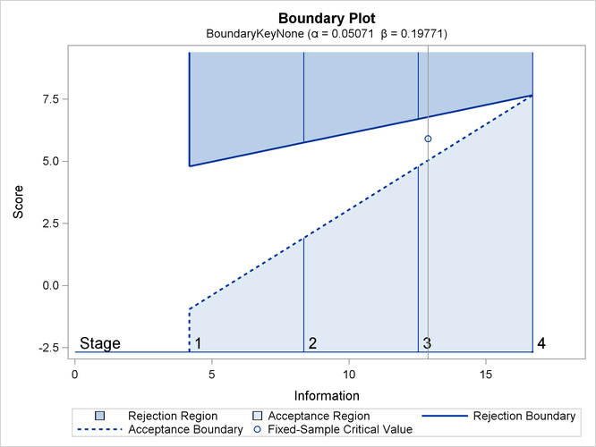
The “Boundary Information” table in Output 83.7.3 displays information level, alternative reference, and boundary values. With the specified BOUNDARYSCALE=SCORE option, the alternative reference and boundary values are displayed with the score statistics scale.
Output 83.7.3: Boundary Information
| Boundary Information (Score Scale) Null Reference = 0 |
|||||
|---|---|---|---|---|---|
| _Stage_ | Alternative | Boundary Values | |||
| Information Level | Reference | Upper | |||
| Proportion | Actual | Upper | Beta | Alpha | |
| 1 | 0.2500 | 4.176597 | 2.89500 | -0.95755 | 4.78775 |
| 2 | 0.5000 | 8.353195 | 5.78999 | 1.91510 | 5.74530 |
| 3 | 0.7500 | 12.52979 | 8.68499 | 4.78775 | 6.70285 |
| 4 | 1.0000 | 16.70639 | 11.57998 | 7.66039 | 7.66039 |
With ODS Graphics enabled, a detailed boundary plot with the rejection and acceptance regions is displayed, as shown in Output 83.7.4.
Output 83.7.4: Boundary Plot
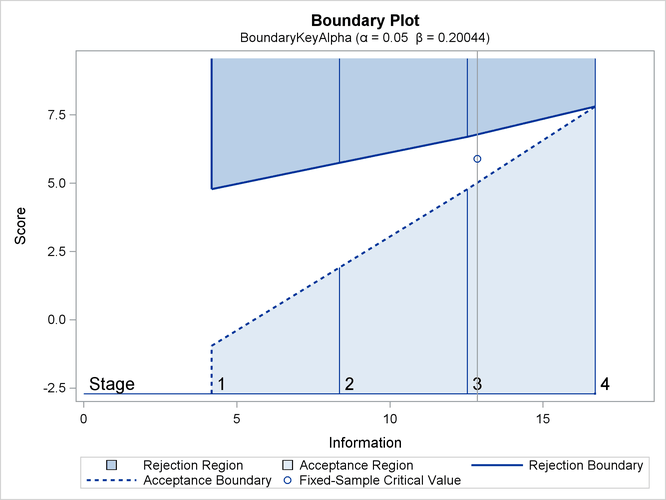
The second design uses the BOUNDARYKEY=ALPHA option to adjust the boundary value at the final stage to maintain the Type I error probability level.
The “Design Information” table in Output 83.7.5 displays design specifications and the derived maximum information. Note that with the BOUNDARYKEY=ALPHA option, the specified
Type I error probability ![]() is maintained.
is maintained.
Output 83.7.5: Whitehead Design Information
| Design Information | |
|---|---|
| Statistic Distribution | Normal |
| Boundary Scale | Score |
| Alternative Hypothesis | Upper |
| Early Stop | Accept/Reject Null |
| Method | Whitehead |
| Boundary Key | Alpha |
| Alternative Reference | 0.693147 |
| Number of Stages | 4 |
| Alpha | 0.05 |
| Beta | 0.20044 |
| Power | 0.79956 |
| Max Information (Percent of Fixed Sample) | 129.9894 |
| Max Information | 16.70639 |
| Null Ref ASN (Percent of Fixed Sample) | 62.6302 |
| Alt Ref ASN (Percent of Fixed Sample) | 74.00064 |
The “Method Information” table in Output 83.7.6 displays the specified and derived ![]() and
and ![]() errors and the derived drift parameter. The derived Type I error probability is the same as the specified
errors and the derived drift parameter. The derived Type I error probability is the same as the specified ![]() and the derived Type II error probability
and the derived Type II error probability ![]() is not the same as the specified
is not the same as the specified ![]() with the BOUNDARYKEY=ALPHA option.
with the BOUNDARYKEY=ALPHA option.
Output 83.7.6: Method Information
| Method Information | |||||||
|---|---|---|---|---|---|---|---|
| Boundary | Method | Alpha | Beta | Whitehead | Alternative Reference |
Drift | |
| Tau | C | ||||||
| Upper Alpha | Whitehead | 0.05000 | . | 0.25 | 4.60517 | 0.693147 | 2.833131 |
| Upper Beta | Whitehead | . | 0.20044 | 0.25 | 4.60517 | 0.693147 | 2.833131 |
The “Boundary Information” table in Output 83.7.7 displays information level, alternative reference, and boundary values.
Output 83.7.7: Boundary Information
| Boundary Information (Score Scale) Null Reference = 0 |
|||||
|---|---|---|---|---|---|
| _Stage_ | Alternative | Boundary Values | |||
| Information Level | Reference | Upper | |||
| Proportion | Actual | Upper | Beta | Alpha | |
| 1 | 0.2500 | 4.176597 | 2.89500 | -0.95755 | 4.78775 |
| 2 | 0.5000 | 8.353195 | 5.78999 | 1.91510 | 5.74530 |
| 3 | 0.7500 | 12.52979 | 8.68499 | 4.78775 | 6.70285 |
| 4 | 1.0000 | 16.70639 | 11.57998 | 7.81300 | 7.81300 |
With ODS Graphics enabled, a detailed boundary plot with the rejection and acceptance regions is displayed, as shown in Output 83.7.8.
Output 83.7.8: Boundary Plot
The third design specifies the BOUNDARYKEY=BETA option to derive the boundary values to maintain the Type II error probability
level ![]() .
.
The “Design Information” table in Output 83.7.9 displays design specifications and the derived maximum information. Note that with the BOUNDARYKEY=BETA option, the specified
Type II error probability ![]() is maintained.
is maintained.
Output 83.7.9: Whitehead Design Information
| Design Information | |
|---|---|
| Statistic Distribution | Normal |
| Boundary Scale | Score |
| Alternative Hypothesis | Upper |
| Early Stop | Accept/Reject Null |
| Method | Whitehead |
| Boundary Key | Beta |
| Alternative Reference | 0.693147 |
| Number of Stages | 4 |
| Alpha | 0.05011 |
| Beta | 0.2 |
| Power | 0.8 |
| Max Information (Percent of Fixed Sample) | 129.9364 |
| Max Information | 16.70639 |
| Null Ref ASN (Percent of Fixed Sample) | 62.60462 |
| Alt Ref ASN (Percent of Fixed Sample) | 73.97042 |
The “Method Information” table in Output 83.7.10 displays the ![]() and
and ![]() errors and the derived drift parameter. The derived Type II error probability is the same as the specified
errors and the derived drift parameter. The derived Type II error probability is the same as the specified ![]() and the derived Type I error probability
and the derived Type I error probability ![]() is not the same as the specified
is not the same as the specified ![]() with the BOUNDARYKEY=BETA option.
with the BOUNDARYKEY=BETA option.
Output 83.7.10: Method Information
| Method Information | |||||||
|---|---|---|---|---|---|---|---|
| Boundary | Method | Alpha | Beta | Whitehead | Alternative Reference |
Drift | |
| Tau | C | ||||||
| Upper Alpha | Whitehead | 0.05011 | . | 0.25 | 4.60517 | 0.693147 | 2.833131 |
| Upper Beta | Whitehead | . | 0.20000 | 0.25 | 4.60517 | 0.693147 | 2.833131 |
The “Boundary Information” table in Output 83.7.11 displays information level, alternative reference, and boundary values.
Output 83.7.11: Boundary Information
| Boundary Information (Score Scale) Null Reference = 0 |
|||||
|---|---|---|---|---|---|
| _Stage_ | Alternative | Boundary Values | |||
| Information Level | Reference | Upper | |||
| Proportion | Actual | Upper | Beta | Alpha | |
| 1 | 0.2500 | 4.176597 | 2.89500 | -0.95755 | 4.78775 |
| 2 | 0.5000 | 8.353195 | 5.78999 | 1.91510 | 5.74530 |
| 3 | 0.7500 | 12.52979 | 8.68499 | 4.78775 | 6.70285 |
| 4 | 1.0000 | 16.70639 | 11.57998 | 7.78899 | 7.78899 |
With ODS Graphics enabled, a detailed boundary plot with the rejection and acceptance regions is displayed, as shown in Output 83.7.12.
Output 83.7.12: Boundary Plot

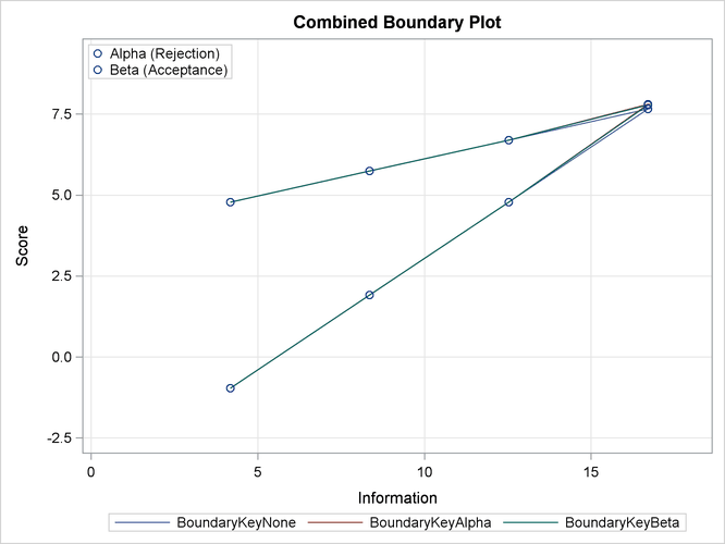
With the PLOTS=COMBINEDBOUNDARY option, a combined plot of group sequential boundaries for all designs is displayed, as shown in Output 83.7.13. It shows that three designs are similar, with a slightly smaller boundary value at the final stage for the design with the BOUNDARYKEY=NONE option.
Output 83.7.13: Combined Boundary Plot
The following statements invoke the SEQDESIGN procedure and specify the SAMPLESIZE statement to derive required sample sizes for a log-rank test comparing two survival distributions for the treatment effect (Jennison and Turnbull 2000, pp. 77–79; Whitehead 1997, pp. 36–39):
proc seqdesign altref=0.693147
               bscale=score
               ;
   BoundaryKeyAlpha: design nstages=4
                            method=whitehead
                            boundarykey=alpha
                            alt=upper   stop=both
                            alpha=0.05  beta=0.20
                            ;
   samplesize model=twosamplesurvival
                    ( nullhazard=0.03466 accrate=10);
run;
The design is identical to the previous design with the BOUNDARYKEY=ALPHA option except with the addition of the sample size computation.
The “Sample Size Summary” table in Output 83.7.14 displays parameters for the sample size computation. Since the ACCTIME= option is not specified for the accrual time, the minimum and maximum accrual times are derived for the specified accrual rate.
Output 83.7.14: Sample Size Summary
| Sample Size Summary | |
|---|---|
| Test | Two-Sample Survival |
| Null Hazard Rate | 0.03466 |
| Hazard Rate (Group A) | 0.01733 |
| Hazard Rate (Group B) | 0.03466 |
| Hazard Ratio | 0.5 |
| log(Hazard Ratio) | -0.69315 |
| Reference Hazards | Alt Ref |
| Accrual | Uniform |
| Accrual Rate | 10 |
| Min Accrual Time | 6.682556 |
| Min Sample Size | 66.82556 |
| Max Accrual Time | 25.40111 |
| Max Sample Size | 254.0111 |
| Max Number of Events | 66.82556 |
If the ACCTIME=20 option is specified in the SAMPLESIZE statement, the “Sample Size Summary” table in Output 83.7.15 also displays the follow-up time and maximum sample size with the specified accrual time.
Output 83.7.15: Sample Size Summary
| Sample Size Summary | |
|---|---|
| Test | Two-Sample Survival |
| Null Hazard Rate | 0.03466 |
| Hazard Rate (Group A) | 0.01733 |
| Hazard Rate (Group B) | 0.03466 |
| Hazard Ratio | 0.5 |
| log(Hazard Ratio) | -0.69315 |
| Reference Hazards | Alt Ref |
| Accrual | Uniform |
| Accrual Rate | 10 |
| Accrual Time | 20 |
| Follow-up Time | 6.474376 |
| Total Time | 26.47438 |
| Max Number of Events | 66.82556 |
| Max Sample Size | 200 |
| Expected Sample Size (Null Ref) | 161.5941 |
| Expected Sample Size (Alt Ref) | 172.4693 |
The “Number of Events (D) and Sample Sizes (N)” table in Output 83.7.16 displays the required time at each stage, in both fractional and integer numbers. The derived times under the heading “Fractional Time” are not integers. These times are rounded up to integers under the heading “Ceiling Time.” The table also displays the numbers of events and sample sizes at each stage.
Output 83.7.16: Number of Events and Sample Sizes
| Numbers of Events (D) and Sample Sizes (N) Two-Sample Log-Rank Test |
||||||||||||||||
|---|---|---|---|---|---|---|---|---|---|---|---|---|---|---|---|---|
| _Stage_ | Fractional Time | Ceiling Time | ||||||||||||||
| D | D(Grp 1) | D(Grp 2) | Time | N | N(Grp 1) | N(Grp 2) | Information | D | D(Grp 1) | D(Grp 2) | Time | N | N(Grp 1) | N(Grp 2) | Information | |
| 1 | 16.71 | 5.82 | 10.89 | 11.9867 | 119.87 | 59.93 | 59.93 | 4.1766 | 16.74 | 5.83 | 10.91 | 12 | 120.00 | 60.00 | 60.00 | 4.1854 |
| 2 | 33.41 | 11.84 | 21.57 | 17.3585 | 173.58 | 86.79 | 86.79 | 8.3532 | 35.73 | 12.68 | 23.04 | 18 | 180.00 | 90.00 | 90.00 | 8.9322 |
| 3 | 50.12 | 18.01 | 32.11 | 21.7480 | 200.00 | 100.00 | 100.00 | 12.5298 | 51.07 | 18.37 | 32.70 | 22 | 200.00 | 100.00 | 100.00 | 12.7667 |
| 4 | 66.83 | 24.46 | 42.37 | 26.4744 | 200.00 | 100.00 | 100.00 | 16.7064 | 68.55 | 25.14 | 43.41 | 27 | 200.00 | 100.00 | 100.00 | 17.1378 |