The SEQDESIGN Procedure
-
Overview

- Getting Started
-
Syntax
-
DetailsFixed-Sample Clinical TrialsOne-Sided Fixed-Sample Tests in Clinical TrialsTwo-Sided Fixed-Sample Tests in Clinical TrialsGroup Sequential MethodsStatistical Assumptions for Group Sequential DesignsBoundary ScalesBoundary VariablesType I and Type II ErrorsUnified Family MethodsHaybittle-Peto MethodWhitehead MethodsError Spending MethodsAcceptance (beta) BoundaryBoundary Adjustments for Overlapping Lower and Upper beta BoundariesSpecified and Derived ParametersApplicable Boundary KeysSample Size ComputationApplicable One-Sample Tests and Sample Size ComputationApplicable Two-Sample Tests and Sample Size ComputationApplicable Regression Parameter Tests and Sample Size ComputationAspects of Group Sequential DesignsSummary of Methods in Group Sequential DesignsTable OutputODS Table NamesGraphics OutputODS Graphics
-
ExamplesCreating Fixed-Sample DesignsCreating a One-Sided O’Brien-Fleming DesignCreating Two-Sided Pocock and O’Brien-Fleming DesignsGenerating Graphics Display for Sequential DesignsCreating Designs Using Haybittle-Peto MethodsCreating Designs with Various Stopping CriteriaCreating Whitehead’s Triangular DesignsCreating a One-Sided Error Spending DesignCreating Designs with Various Number of StagesCreating Two-Sided Error Spending Designs with and without Overlapping Lower and Upper beta BoundariesCreating a Two-Sided Asymmetric Error Spending Design with Early Stopping to Reject H0Creating a Two-Sided Asymmetric Error Spending Design with Early Stopping to Reject or Accept H0Creating a Design with a Nonbinding Beta BoundaryComputing Sample Size for Survival Data
- References
Example 83.5 Creating Designs Using Haybittle-Peto Methods
This example requests two 3-stage group sequential designs for normally distributed statistics. Each design uses a Haybittle-Peto
method with a two-sided alternative and early stopping to reject the hypothesis. One design uses the specified interim boundary
Z values and derives the final-stage boundary value for the specified ![]() and
and ![]() errors. The other design uses the specified boundary Z values and derives the overall
errors. The other design uses the specified boundary Z values and derives the overall ![]() and
and ![]() errors.
errors.
The following statements specify the interim boundary Z values and derive the final-stage boundary value for the specified ![]() and
and ![]() :
:
ods graphics on;
proc seqdesign altref=0.25
               errspend
               stopprob
               plots=errspend
               ;
   OneSidedPeto: design nstages=3
                 method=peto( z=3)
                 alt=upper   stop=reject
                 alpha=0.05  beta=0.10;
run;
ods graphics off;
The “Design Information” table in Output 83.5.1 displays design specifications and maximum information in percentage of its corresponding fixed-sample design.
Output 83.5.1: Haybittle-Peto Design Information
| Design Information | |
|---|---|
| Statistic Distribution | Normal |
| Boundary Scale | Standardized Z |
| Alternative Hypothesis | Upper |
| Early Stop | Reject Null |
| Method | Haybittle-Peto |
| Boundary Key | Both |
| Alternative Reference | 0.25 |
| Number of Stages | 3 |
| Alpha | 0.05 |
| Beta | 0.1 |
| Power | 0.9 |
| Max Information (Percent of Fixed Sample) | 100.2466 |
| Max Information | 137.3592 |
| Null Ref ASN (Percent of Fixed Sample) | 100.1192 |
| Alt Ref ASN (Percent of Fixed Sample) | 87.35 |
The “Method Information” table in Output 83.5.2 displays the ![]() and
and ![]() errors and the derived drift parameter, which is the standardized alternative reference at the final stage.
errors and the derived drift parameter, which is the standardized alternative reference at the final stage.
Output 83.5.2: Method Information
| Method Information | |||||
|---|---|---|---|---|---|
| Boundary | Method | Alpha | Beta | Alternative Reference |
Drift |
| Upper Alpha | Haybittle-Peto | 0.05000 | 0.10000 | 0.25 | 2.930009 |
With the STOPPROB option, the “Expected Cumulative Stopping Probabilities” table in Output 83.5.3 displays the expected stopping stage and cumulative stopping probability to reject the null hypothesis at each stage under
various hypothetical references ![]() , where
, where ![]() is the alternative reference and
is the alternative reference and ![]() are the default values in the CREF= option.
are the default values in the CREF= option.
Output 83.5.3: Stopping Probabilities
| Expected Cumulative Stopping Probabilities Reference = CRef * (Alt Reference) |
|||||
|---|---|---|---|---|---|
| CRef | Expected Stopping Stage |
Source | Stopping Probabilities | ||
| Stage_1 | Stage_2 | Stage_3 | |||
| 0.0000 | 2.996 | Reject Null | 0.00135 | 0.00246 | 0.05000 |
| 0.5000 | 2.941 | Reject Null | 0.01561 | 0.04372 | 0.42762 |
| 1.0000 | 2.614 | Reject Null | 0.09538 | 0.29057 | 0.90000 |
| 1.5000 | 1.944 | Reject Null | 0.32185 | 0.73442 | 0.99698 |
The “Boundary Information” table in Output 83.5.4 displays information level, alternative references, and boundary values. By default (or equivalently if you specify BOUNDARYSCALE=STDZ),
the standardized Z scale is used to display the alternative references and boundary values. The resulting standardized alternative reference
at stage k is given by ![]() , where
, where ![]() is the alternative reference and
is the alternative reference and ![]() is the information level at stage k,
is the information level at stage k, ![]() .
.
Output 83.5.4: Boundary Information
| Boundary Information (Standardized Z Scale) Null Reference = 0 |
||||
|---|---|---|---|---|
| _Stage_ | Alternative | Boundary Values | ||
| Information Level | Reference | Upper | ||
| Proportion | Actual | Upper | Alpha | |
| 1 | 0.3333 | 45.7864 | 1.69164 | 3.00000 |
| 2 | 0.6667 | 91.57281 | 2.39234 | 3.00000 |
| 3 | 1.0000 | 137.3592 | 2.93001 | 1.65042 |
At each interim stage, if the standardized statistic ![]() , the trial is stopped and the null hypothesis is rejected. If the statistic
, the trial is stopped and the null hypothesis is rejected. If the statistic ![]() , the trial continues to the next stage. At the final stage, the null hypothesis is rejected if the statistic
, the trial continues to the next stage. At the final stage, the null hypothesis is rejected if the statistic ![]() . Otherwise, the hypothesis is accepted. Note that the boundary values at the final stage, 1.65, are close to the critical
values 1.645 in the corresponding fixed-sample design.
. Otherwise, the hypothesis is accepted. Note that the boundary values at the final stage, 1.65, are close to the critical
values 1.645 in the corresponding fixed-sample design.
The “Error Spending Information” in Output 83.5.5 displays cumulative error spending at each stage for each boundary. The stage 1 ![]() spending 0.00135 corresponds to the one-sided p-value for a standardized Z statistic,
spending 0.00135 corresponds to the one-sided p-value for a standardized Z statistic, ![]() .
.
Output 83.5.5: Error Spending Information
| Error Spending Information | |||
|---|---|---|---|
| _Stage_ | Information Level |
Cumulative Error Spending | |
| Upper | |||
| Proportion | Beta | Alpha | |
| 1 | 0.3333 | 0.00000 | 0.00135 |
| 2 | 0.6667 | 0.00000 | 0.00246 |
| 3 | 1.0000 | 0.10000 | 0.05000 |
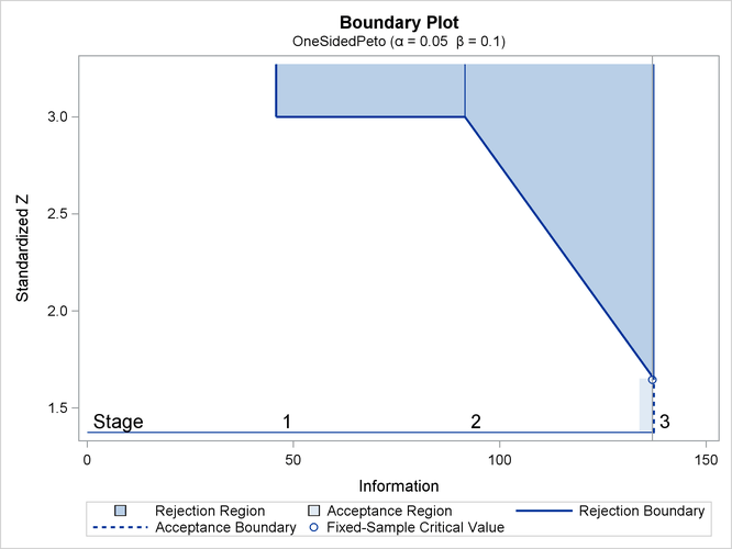
With ODS Graphics enabled, a detailed boundary plot with the rejection and acceptance regions is displayed, as shown in Output 83.5.6. With the STOP=REJECT option, the interim rejection boundaries are displayed.
Output 83.5.6: Boundary Plot
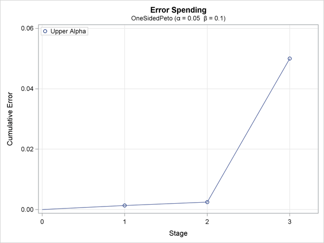
With the PLOTS=ERRSPEND option, the procedure displays a plot of error spending for each boundary, as shown in Output 83.5.7. The error spending values in the “Error Spending Information” in Output 83.5.4 are displayed in the plot. As expected, the error spending at each of the first two stages is small, with the standardized Z boundary value 3.
Output 83.5.7: Error Spending Plot
The following statements specify the boundary Z values and derive the ![]() and
and ![]() errors from these completely specified boundary values:
errors from these completely specified boundary values:
ods graphics on;
proc seqdesign altref=0.25
               maxinfo=200
               errspend
               stopprob
               plots=errspend
               ;
   OneSidedPeto: design nstages=3
                 method=peto(z=3 2.5 2)
                 alt=upper  stop=reject
                 boundarykey=none
                 ;
run;
ods graphics off;
The “Design Information” table in Output 83.5.8 displays design specifications and derived ![]() and
and ![]() error levels.
error levels.
Output 83.5.8: Design Information
| Design Information | |
|---|---|
| Statistic Distribution | Normal |
| Boundary Scale | Standardized Z |
| Alternative Hypothesis | Upper |
| Early Stop | Reject Null |
| Method | Haybittle-Peto |
| Boundary Key | None |
| Alternative Reference | 0.25 |
| Number of Stages | 3 |
| Alpha | 0.02532 |
| Beta | 0.06035 |
| Power | 0.93965 |
| Max Information (Percent of Fixed Sample) | 101.6769 |
| Max Information | 200 |
| Null Ref ASN (Percent of Fixed Sample) | 101.3933 |
| Alt Ref ASN (Percent of Fixed Sample) | 73.74031 |
The “Method Information” table in Output 83.5.9 displays the ![]() and
and ![]() errors and the derived drift parameter for each boundary.
errors and the derived drift parameter for each boundary.
Output 83.5.9: Method Information
| Method Information | |||||
|---|---|---|---|---|---|
| Boundary | Method | Alpha | Beta | Alternative Reference |
Drift |
| Upper Alpha | Haybittle-Peto | 0.02532 | 0.06035 | 0.25 | 3.535534 |
With the STOPPROB option, the “Expected Cumulative Stopping Probabilities” table in Output 83.5.10 displays the expected stopping stage and cumulative stopping probability to reject the null hypothesis at each stage under
various hypothetical references ![]() , where
, where ![]() is the alternative reference and
is the alternative reference and ![]() are the default values in the CREF= option.
are the default values in the CREF= option.
Output 83.5.10: Stopping Probabilities
| Expected Cumulative Stopping Probabilities Reference = CRef * (Alt Reference) |
|||||
|---|---|---|---|---|---|
| CRef | Expected Stopping Stage |
Source | Stopping Probabilities | ||
| Stage_1 | Stage_2 | Stage_3 | |||
| 0.0000 | 2.992 | Reject Null | 0.00135 | 0.00702 | 0.02532 |
| 0.5000 | 2.826 | Reject Null | 0.02389 | 0.15030 | 0.41775 |
| 1.0000 | 2.176 | Reject Null | 0.16884 | 0.65544 | 0.93965 |
| 1.5000 | 1.508 | Reject Null | 0.52466 | 0.96708 | 0.99954 |
The “Boundary Information” table in Output 83.5.11 displays information level, alternative references, and boundary values.
Output 83.5.11: Boundary Information
| Boundary Information (Standardized Z Scale) Null Reference = 0 |
||||
|---|---|---|---|---|
| _Stage_ | Alternative | Boundary Values | ||
| Information Level | Reference | Upper | ||
| Proportion | Actual | Upper | Alpha | |
| 1 | 0.3333 | 66.66667 | 2.04124 | 3.00000 |
| 2 | 0.6667 | 133.3333 | 2.88675 | 2.50000 |
| 3 | 1.0000 | 200 | 3.53553 | 2.00000 |
The “Error Spending Information” in Output 83.5.12 displays cumulative error spending at each stage for each boundary. The first-stage ![]() spending 0.00135 corresponds to the one-sided p-value for a standardized Z statistic,
spending 0.00135 corresponds to the one-sided p-value for a standardized Z statistic, ![]() .
.
Output 83.5.12: Error Spending Information
| Error Spending Information | |||
|---|---|---|---|
| _Stage_ | Information Level |
Cumulative Error Spending | |
| Upper | |||
| Proportion | Beta | Alpha | |
| 1 | 0.3333 | 0.00000 | 0.00135 |
| 2 | 0.6667 | 0.00000 | 0.00702 |
| 3 | 1.0000 | 0.06035 | 0.02532 |
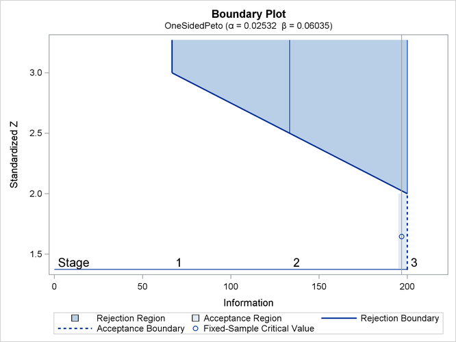
With ODS Graphics enabled, a detailed boundary plot with the rejection and acceptance regions is displayed, as shown in Output 83.5.13. With the STOP=REJECT option, the interim rejection boundaries are displayed.
Output 83.5.13: Boundary Plot
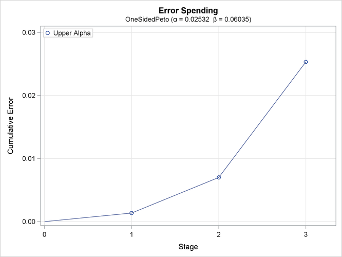
With the PLOTS=ERRSPEND option, the procedure displays a plot of error spending for each boundary, as shown in Output 83.5.14. The error spending values in the “Error Spending Information” table in Output 83.5.10 are displayed in the plot.
Output 83.5.14: Error Spending Plot