The PLS Procedure

Spectrometric Calibration
The example in this section illustrates basic features of the PLS procedure. The data are reported in Umetrics (1995); the original source is Lindberg, Persson, and Wold (1983). Suppose that you are researching pollution in the Baltic Sea, and you would like to use the spectra of samples of seawater
to determine the amounts of three compounds present in samples from the Baltic Sea: lignin sulfonate (ls: pulp industry pollution), humic acids (ha: natural forest products), and optical whitener from detergent (dt). Spectrometric calibration is a type of problem in which partial least squares can be very effective. The predictors are
the spectra emission intensities at different frequencies in sample spectrum, and the responses are the amounts of various
chemicals in the sample.
For the purposes of calibrating the model, samples with known compositions are used. The calibration data consist of 16 samples
of known concentrations of ls, ha, and dt, with spectra based on 27 frequencies (or, equivalently, wavelengths). The following statements create a SAS data set named
Sample for these data.
data Sample;
   input obsnam $ v1-v27 ls ha dt @@;
   datalines;
EM1   2766 2610 3306 3630 3600 3438 3213 3051 2907 2844 2796
      2787 2760 2754 2670 2520 2310 2100 1917 1755 1602 1467
      1353 1260 1167 1101 1017         3.0110  0.0000   0.00
EM2   1492 1419 1369 1158  958  887  905  929  920  887  800
       710  617  535  451  368  296  241  190  157  128  106
        89   70   65   56   50         0.0000  0.4005   0.00
EM3   2450 2379 2400 2055 1689 1355 1109  908  750  673  644
       640  630  618  571  512  440  368  305  247  196  156
       120   98   80   61   50         0.0000  0.0000  90.63
EM4   2751 2883 3492 3570 3282 2937 2634 2370 2187 2070 2007
      1974 1950 1890 1824 1680 1527 1350 1206 1080  984  888
       810  732  669  630  582         1.4820  0.1580  40.00
EM5   2652 2691 3225 3285 3033 2784 2520 2340 2235 2148 2094
      2049 2007 1917 1800 1650 1464 1299 1140 1020  909  810
       726  657  594  549  507         1.1160  0.4104  30.45
EM6   3993 4722 6147 6720 6531 5970 5382 4842 4470 4200 4077
      4008 3948 3864 3663 3390 3090 2787 2481 2241 2028 1830
      1680 1533 1440 1314 1227         3.3970  0.3032  50.82
EM7   4032 4350 5430 5763 5490 4974 4452 3990 3690 3474 3357
      3300 3213 3147 3000 2772 2490 2220 1980 1779 1599 1440
      1320 1200 1119 1032  957         2.4280  0.2981  70.59
EM8   4530 5190 6910 7580 7510 6930 6150 5490 4990 4670 4490
      4370 4300 4210 4000 3770 3420 3060 2760 2490 2230 2060
      1860 1700 1590 1490 1380         4.0240  0.1153  89.39
EM9   4077 4410 5460 5857 5607 5097 4605 4170 3864 3708 3588
      3537 3480 3330 3192 2910 2610 2325 2064 1830 1638 1476
      1350 1236 1122 1044  963         2.2750  0.5040  81.75
EM10  3450 3432 3969 4020 3678 3237 2814 2487 2205 2061 2001
      1965 1947 1890 1776 1635 1452 1278 1128  981  867  753
       663  600  552  507  468         0.9588  0.1450 101.10
EM11  4989 5301 6807 7425 7155 6525 5784 5166 4695 4380 4197
      4131 4077 3972 3777 3531 3168 2835 2517 2244 2004 1809
      1620 1470 1359 1266 1167         3.1900  0.2530 120.00
EM12  5340 5790 7590 8390 8310 7670 6890 6190 5700 5380 5200
      5110 5040 4900 4700 4390 3970 3540 3170 2810 2490 2240
      2060 1870 1700 1590 1470         4.1320  0.5691 117.70
EM13  3162 3477 4365 4650 4470 4107 3717 3432 3228 3093 3009
      2964 2916 2838 2694 2490 2253 2013 1788 1599 1431 1305
      1194 1077  990  927  855         2.1600  0.4360  27.59
EM14  4380 4695 6018 6510 6342 5760 5151 4596 4200 3948 3807
      3720 3672 3567 3438 3171 2880 2571 2280 2046 1857 1680
      1548 1413 1314 1200 1119         3.0940  0.2471  61.71
EM15  4587 4200 5040 5289 4965 4449 3939 3507 3174 2970 2850
      2814 2748 2670 2529 2328 2088 1851 1641 1431 1284 1134
      1020  918  840  756  714         1.6040  0.2856 108.80
EM16  4017 4725 6090 6570 6354 5895 5346 4911 4611 4422 4314
      4287 4224 4110 3915 3600 3240 2913 2598 2325 2088 1917
      1734 1587 1452 1356 1257         3.1620  0.7012  60.00
;
Fitting a PLS Model
To isolate a few underlying spectral factors that provide a good predictive model, you can fit a PLS model to the 16 samples by using the following SAS statements:
proc pls data=sample;
   model ls ha dt = v1-v27;
run;
By default, the PLS procedure extracts at most 15 factors. The procedure lists the amount of variation accounted for by each of these factors, both individual and cumulative; this listing is shown in Figure 70.1.
Figure 70.1: PLS Variation Summary
| Percent Variation Accounted for by Partial Least Squares Factors |
||||
|---|---|---|---|---|
| Number of Extracted Factors |
Model Effects | Dependent Variables | ||
| Current | Total | Current | Total | |
| 1 | 97.4607 | 97.4607 | 41.9155 | 41.9155 |
| 2 | 2.1830 | 99.6436 | 24.2435 | 66.1590 |
| 3 | 0.1781 | 99.8217 | 24.5339 | 90.6929 |
| 4 | 0.1197 | 99.9414 | 3.7898 | 94.4827 |
| 5 | 0.0415 | 99.9829 | 1.0045 | 95.4873 |
| 6 | 0.0106 | 99.9935 | 2.2808 | 97.7681 |
| 7 | 0.0017 | 99.9952 | 1.1693 | 98.9374 |
| 8 | 0.0010 | 99.9961 | 0.5041 | 99.4415 |
| 9 | 0.0014 | 99.9975 | 0.1229 | 99.5645 |
| 10 | 0.0010 | 99.9985 | 0.1103 | 99.6747 |
| 11 | 0.0003 | 99.9988 | 0.1523 | 99.8270 |
| 12 | 0.0003 | 99.9991 | 0.1291 | 99.9561 |
| 13 | 0.0002 | 99.9994 | 0.0312 | 99.9873 |
| 14 | 0.0004 | 99.9998 | 0.0065 | 99.9938 |
| 15 | 0.0002 | 100.0000 | 0.0062 | 100.0000 |
Note that all of the variation in both the predictors and the responses is accounted for by only 15 factors; this is because there are only 16 sample observations. More important, almost all of the variation is accounted for with even fewer factors—one or two for the predictors and three to eight for the responses.
Selecting the Number of Factors by Cross Validation
A PLS model is not complete until you choose the number of factors. You can choose the number of factors by using cross validation, in which the data set is divided into two or more groups. You fit the model to all groups except one, and then you check the capability of the model to predict responses for the group omitted. Repeating this for each group, you then can measure the overall capability of a given form of the model. The predicted residual sum of squares (PRESS) statistic is based on the residuals generated by this process.
To select the number of extracted factors by cross validation, you specify the CV= option with an argument that says which cross validation method to use. For example, a common method is split-sample validation, in which the different groups are composed of every nth observation beginning with the first, every nth observation beginning with the second, and so on. You can use the CV=SPLIT option to specify split-sample validation with n = 7 by default, as in the following SAS statements:
proc pls data=sample cv=split;
   model ls ha dt = v1-v27;
run;
The resulting output is shown in Figure 70.2 and Figure 70.3.
Figure 70.2: Split-Sample Validated PRESS Statistics for Number of Factors
| Split-sample Validation for the Number of Extracted Factors |
|
|---|---|
| Number of Extracted Factors |
Root Mean PRESS |
| 0 | 1.107747 |
| 1 | 0.957983 |
| 2 | 0.931314 |
| 3 | 0.520222 |
| 4 | 0.530501 |
| 5 | 0.586786 |
| 6 | 0.475047 |
| 7 | 0.477595 |
| 8 | 0.483138 |
| 9 | 0.485739 |
| 10 | 0.48946 |
| 11 | 0.521445 |
| 12 | 0.525653 |
| 13 | 0.531049 |
| 14 | 0.531049 |
| 15 | 0.531049 |
| Minimum root mean PRESS | 0.4750 |
|---|---|
| Minimizing number of factors | 6 |
Figure 70.3: PLS Variation Summary for Split-Sample Validated Model
| Percent Variation Accounted for by Partial Least Squares Factors |
||||
|---|---|---|---|---|
| Number of Extracted Factors |
Model Effects | Dependent Variables | ||
| Current | Total | Current | Total | |
| 1 | 97.4607 | 97.4607 | 41.9155 | 41.9155 |
| 2 | 2.1830 | 99.6436 | 24.2435 | 66.1590 |
| 3 | 0.1781 | 99.8217 | 24.5339 | 90.6929 |
| 4 | 0.1197 | 99.9414 | 3.7898 | 94.4827 |
| 5 | 0.0415 | 99.9829 | 1.0045 | 95.4873 |
| 6 | 0.0106 | 99.9935 | 2.2808 | 97.7681 |
The absolute minimum PRESS is achieved with six extracted factors. Notice, however, that this is not much smaller than the PRESS for three factors. By using the CVTEST option, you can perform a statistical model comparison suggested by van der Voet (1994) to test whether this difference is significant, as shown in the following SAS statements:
proc pls data=sample cv=split cvtest(seed=12345);
   model ls ha dt = v1-v27;
run;
The model comparison test is based on a rerandomization of the data. By default, the seed for this randomization is based on the system clock, but it is specified here. The resulting output is shown in Figure 70.4 and Figure 70.5.
Figure 70.4: Testing Split-Sample Validation for Number of Factors
| Split-sample Validation for the Number of Extracted Factors |
|||
|---|---|---|---|
| Number of Extracted Factors |
Root Mean PRESS | T**2 | Prob > T**2 |
| 0 | 1.107747 | 9.272858 | 0.0010 |
| 1 | 0.957983 | 10.62305 | <.0001 |
| 2 | 0.931314 | 8.950878 | 0.0010 |
| 3 | 0.520222 | 5.133259 | 0.1440 |
| 4 | 0.530501 | 5.168427 | 0.1340 |
| 5 | 0.586786 | 6.437266 | 0.0150 |
| 6 | 0.475047 | 0 | 1.0000 |
| 7 | 0.477595 | 2.809763 | 0.4750 |
| 8 | 0.483138 | 7.189526 | 0.0110 |
| 9 | 0.485739 | 7.931726 | 0.0070 |
| 10 | 0.48946 | 6.612597 | 0.0150 |
| 11 | 0.521445 | 6.666235 | 0.0130 |
| 12 | 0.525653 | 7.092861 | 0.0080 |
| 13 | 0.531049 | 7.538298 | 0.0030 |
| 14 | 0.531049 | 7.538298 | 0.0030 |
| 15 | 0.531049 | 7.538298 | 0.0030 |
| Minimum root mean PRESS | 0.4750 |
|---|---|
| Minimizing number of factors | 6 |
| Smallest number of factors with p > 0.1 | 3 |
Figure 70.5: PLS Variation Summary for Tested Split-Sample Validated Model
| Percent Variation Accounted for by Partial Least Squares Factors |
||||
|---|---|---|---|---|
| Number of Extracted Factors |
Model Effects | Dependent Variables | ||
| Current | Total | Current | Total | |
| 1 | 97.4607 | 97.4607 | 41.9155 | 41.9155 |
| 2 | 2.1830 | 99.6436 | 24.2435 | 66.1590 |
| 3 | 0.1781 | 99.8217 | 24.5339 | 90.6929 |
The p-value of 0.1430 in comparing the cross validated residuals from models with 6 and 3 factors indicates that the difference between the two models is insignificant; therefore, the model with fewer factors is preferred. The variation summary shows that over 99% of the predictor variation and over 90% of the response variation are accounted for by the three factors.
Predicting New Observations
Now that you have chosen a three-factor PLS model for predicting pollutant concentrations based on sample spectra, suppose that you have two new samples. The following SAS statements create a data set containing the spectra for the new samples:
data newobs;
   input obsnam $ v1-v27 @@;
   datalines;
EM17  3933 4518 5637 6006 5721 5187 4641 4149 3789
      3579 3447 3381 3327 3234 3078 2832 2571 2274
      2040 1818 1629 1470 1350 1245 1134 1050  987
EM25  2904 2997 3255 3150 2922 2778 2700 2646 2571
      2487 2370 2250 2127 2052 1713 1419 1200  984
       795  648  525  426  351  291  240  204  162
;
You can apply the PLS model to these samples to estimate pollutant concentration. To do so, append the new samples to the original 16, and specify that the predicted values for all 18 be output to a data set, as shown in the following statements:
data all;
   set sample newobs;
run;

proc pls data=all nfac=3;
   model ls ha dt = v1-v27;
   output out=pred p=p_ls p_ha p_dt;
run;
proc print data=pred;
   where (obsnam in ('EM17','EM25'));
   var obsnam p_ls p_ha p_dt;
run;
The new observations are not used in calculating the PLS model, since they have no response values. Their predicted concentrations are shown in Figure 70.6.
Figure 70.6: Predicted Concentrations for New Observations
| Obs | obsnam | p_ls | p_ha | p_dt |
|---|---|---|---|---|
| 17 | EM17 | 2.54261 | 0.31877 | 81.4174 |
| 18 | EM25 | -0.24716 | 1.37892 | 46.3212 |
Finally, if ODS Graphics is enabled, PLS also displays by default a plot of the amount of variation accounted for by each factor, as well as a correlations loading plot that summarizes the first two dimensions of the PLS model. The following statements, which are the same as the previous split-sample validation analysis but with ODS Graphics enabled, additionally produce Figure 70.7 and Figure 70.8:
ods graphics on;

proc pls data=sample cv=split cvtest(seed=12345);
   model ls ha dt = v1-v27;
run;

ods graphics off;
Figure 70.7: Split-Sample Cross Validation Plot
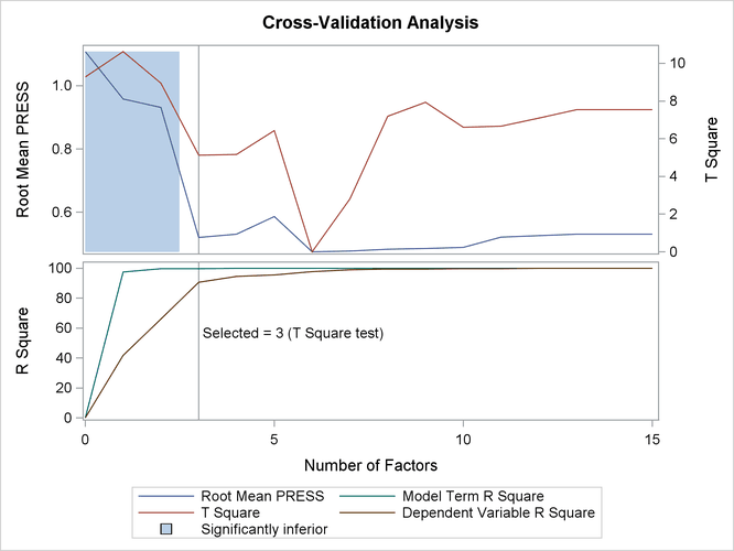
Figure 70.8: Correlation Loadings Plot
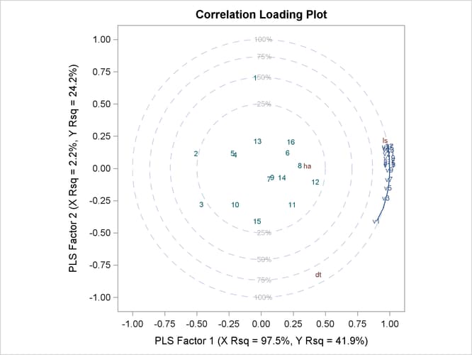
The cross validation plot in Figure 70.7 gives a visual representation of the selection of the optimum number of factors discussed previously. The correlation loadings plot is a compact summary of many features of the PLS model. For example, it shows that the first factor is highly positively correlated with all spectral values, indicating that it is approximately an average of them all; the second factor is positively correlated with the lowest frequencies and negatively correlated with the highest, indicating that it is approximately a contrast between the two ends of the spectrum. The observations, represented by their number in the data set on this plot, are generally spaced well apart, indicating that the data give good information about these first two factors. For more details on the interpretation of the correlation loadings plot, see the section ODS Graphics and Example 70.1.