The MDS Procedure

Example 56.1 Jacobowitz Body Parts Data from Children and Adults
Jacobowitz (1975) collected conditional rank-order data regarding perceived similarity of parts of the body from children of ages 6, 8, and 10 years and from college sophomores. The data set includes data from 15 children (6-year-olds) and 15 sophomores. The method of data collection and some results of an analysis are also described by Young (1987, pp. 4–10). The following statements create the input data set:
data body;
   title  'Jacobowitz Body Parts Data from 6-Year-Olds and Adults';
   title2 'First 15 Subjects (obs 1-225) Are Children';
   title3 'Second 15 Subjects (obs 226-450) Are Adults';
   input  (Cheek Face Mouth Head Ear Body Arm Elbow Hand
           Palm Finger Leg Knee Foot Toe) (2.);
   if _n_ <= 225 then Subject='C'; else subject='A';
   datalines;
 0  2  1  3  4 10  5  9  6  7  8 11 12 13 14
 2  0 12  1 13  3  8 10 11  9  7  4  5  6 14
 3  2  0  1  4  9  5 11  6  7  8 10 13 12 14
 2  1  3  0  4  9  5  6 11  7  8 10 12 13 14

   ... more lines ...

10 12 11 13  9 14  8  7  4  6  2  3  5  1  0
;
The data are analyzed as row conditional (CONDITION=ROW) at the ordinal level of measurement (LEVEL=ORDINAL) by using the weighted Euclidean model (COEF=DIAGONAL) in three dimensions (DIMENSION=3). The final estimates are displayed (PFINAL). The estimates (OUT=OUT) and fitted values (OUTRES=RES) are saved in output data sets. The following statements produce Output 56.1.1:
ods graphics on;

proc mds data=body condition=row level=ordinal coef=diagonal
         dimension=3 pfinal out=out outres=res;
   subject subject;
   title5 'Nonmetric Weighted MDS';
run;
Output 56.1.1: Analysis of Body Parts Data
| Jacobowitz Body Parts Data from 6-Year-Olds and Adults |
| First 15 Subjects (obs 1-225) Are Children |
| Second 15 Subjects (obs 226-450) Are Adults |
| Nonmetric Weighted MDS |
| Iteration | Type | Badness- of-Fit Criterion |
Change in Criterion |
Convergence Measures | |
|---|---|---|---|---|---|
| Monotone | Gradient | ||||
| 0 | Initial | 0.5938 | . | . | . |
| 1 | Monotone | 0.2344 | 0.3594 | 0.4693 | 0.4028 |
| 2 | Gau-New | 0.2080 | 0.0264 | . | . |
| 3 | Monotone | 0.1963 | 0.0118 | 0.0556 | 0.2630 |
| 4 | Gau-New | 0.1927 | 0.003592 | . | . |
| 5 | Monotone | 0.1797 | 0.0130 | 0.0463 | 0.1544 |
| 6 | Gau-New | 0.1779 | 0.001809 | . | . |
| 7 | Monotone | 0.1744 | 0.003430 | 0.0225 | 0.1210 |
| 8 | Gau-New | 0.1736 | 0.000807 | . | . |
| 9 | Monotone | 0.1717 | 0.001929 | 0.0161 | 0.1128 |
| 10 | Gau-New | 0.1712 | 0.000474 | . | . |
| 11 | Monotone | 0.1698 | 0.001413 | 0.0135 | 0.1119 |
| 12 | Gau-New | 0.1696 | 0.000188 | . | . |
| 13 | Monotone | 0.1684 | 0.001261 | 0.0121 | 0.1121 |
| 14 | Gau-New | 0.1683 | 0.000117 | . | . |
| 15 | Monotone | 0.1672 | 0.001096 | 0.0111 | 0.1064 |
| 16 | Gau-New | 0.1670 | 0.000131 | . | . |
| 17 | Monotone | 0.1661 | 0.000902 | 0.0103 | 0.0965 |
| 18 | Gau-New | 0.1660 | 0.000160 | . | . |
| 19 | Monotone | 0.1652 | 0.000736 | 0.009740 | 0.0980 |
| 20 | Gau-New | 0.1651 | 0.000169 | . | 0.1062 |
| 21 | Gau-New | 0.1645 | 0.000542 | . | 0.0161 |
| 22 | Gau-New | 0.1645 | 4.2645E-6 | . | 0.009969 |
| Convergence criteria are satisfied. |
| Configuration | |||
|---|---|---|---|
| Dim1 | Dim2 | Dim3 | |
| Cheek | 0.25 | 1.47 | 2.06 |
| Face | 0.36 | 0.32 | 0.33 |
| Mouth | 0.78 | 0.08 | 1.08 |
| Head | 2.10 | 1.07 | -0.01 |
| Ear | 0.26 | 0.72 | -0.34 |
| Body | 1.51 | -0.61 | -0.68 |
| Arm | -0.74 | 2.07 | -0.59 |
| Elbow | -0.51 | -0.21 | 0.01 |
| Hand | 0.46 | -1.50 | -0.60 |
| Palm | -1.44 | -0.81 | 1.48 |
| Finger | -0.24 | -0.24 | -0.81 |
| Leg | -1.68 | 0.26 | -0.05 |
| Knee | -1.19 | -1.19 | -1.36 |
| Foot | 0.16 | -0.03 | -1.56 |
| Toe | -0.10 | -1.39 | 1.02 |
| Dimension Coefficients | |||
|---|---|---|---|
| Subject | 1 | 2 | 3 |
| C | 1.00 | 1.12 | 0.86 |
| C | 0.96 | 1.02 | 1.01 |
| C | 0.98 | 1.05 | 0.98 |
| C | 1.02 | 1.08 | 0.89 |
| C | 0.95 | 1.04 | 1.01 |
| C | 0.99 | 1.12 | 0.89 |
| C | 1.07 | 1.00 | 0.93 |
| C | 1.04 | 1.02 | 0.94 |
| C | 0.99 | 1.15 | 0.83 |
| C | 0.89 | 1.11 | 0.99 |
| C | 1.04 | 1.03 | 0.92 |
| C | 1.06 | 1.01 | 0.93 |
| C | 0.92 | 1.24 | 0.78 |
| C | 0.97 | 0.98 | 1.05 |
| C | 1.03 | 1.00 | 0.97 |
| A | 0.93 | 1.17 | 0.88 |
| A | 0.89 | 1.12 | 0.97 |
| A | 0.88 | 1.17 | 0.94 |
| A | 0.81 | 1.14 | 1.02 |
| A | 0.90 | 1.11 | 0.98 |
| A | 0.90 | 1.17 | 0.91 |
| A | 0.92 | 1.17 | 0.88 |
| A | 0.97 | 1.19 | 0.80 |
| A | 0.95 | 1.16 | 0.87 |
| A | 1.08 | 1.07 | 0.83 |
| A | 0.95 | 1.20 | 0.81 |
| A | 1.00 | 0.97 | 1.02 |
| A | 0.89 | 1.18 | 0.91 |
| A | 0.97 | 1.15 | 0.86 |
| A | 0.93 | 1.21 | 0.82 |
| Subject | Number of Nonmissing Data |
Weight | Badness-of-Fit Criterion | Distance Correlation | Uncorrected Distance Correlation |
|---|---|---|---|---|---|
| C | 160 | 0.03 | 0.15 | 0.86 | 0.99 |
| C | 163 | 0.03 | 0.19 | 0.78 | 0.98 |
| C | 166 | 0.03 | 0.20 | 0.79 | 0.98 |
| C | 158 | 0.03 | 0.16 | 0.84 | 0.99 |
| C | 173 | 0.03 | 0.18 | 0.83 | 0.98 |
| C | 164 | 0.03 | 0.14 | 0.90 | 0.99 |
| C | 158 | 0.03 | 0.20 | 0.77 | 0.98 |
| C | 170 | 0.03 | 0.18 | 0.83 | 0.98 |
| C | 156 | 0.03 | 0.15 | 0.88 | 0.99 |
| C | 165 | 0.03 | 0.18 | 0.79 | 0.98 |
| C | 153 | 0.03 | 0.19 | 0.79 | 0.98 |
| C | 162 | 0.03 | 0.17 | 0.83 | 0.98 |
| C | 161 | 0.03 | 0.14 | 0.90 | 0.99 |
| C | 164 | 0.03 | 0.17 | 0.83 | 0.99 |
| C | 161 | 0.03 | 0.18 | 0.81 | 0.98 |
| A | 163 | 0.03 | 0.15 | 0.87 | 0.99 |
| A | 174 | 0.04 | 0.17 | 0.85 | 0.99 |
| A | 172 | 0.03 | 0.15 | 0.89 | 0.99 |
| A | 175 | 0.04 | 0.17 | 0.85 | 0.98 |
| A | 171 | 0.03 | 0.15 | 0.87 | 0.99 |
| A | 163 | 0.03 | 0.16 | 0.86 | 0.99 |
| A | 173 | 0.03 | 0.14 | 0.90 | 0.99 |
| A | 160 | 0.03 | 0.14 | 0.89 | 0.99 |
| A | 164 | 0.03 | 0.14 | 0.90 | 0.99 |
| A | 158 | 0.03 | 0.16 | 0.86 | 0.99 |
| A | 165 | 0.03 | 0.16 | 0.87 | 0.99 |
| A | 168 | 0.03 | 0.18 | 0.82 | 0.98 |
| A | 175 | 0.04 | 0.15 | 0.89 | 0.99 |
| A | 172 | 0.03 | 0.16 | 0.88 | 0.99 |
| A | 175 | 0.04 | 0.15 | 0.90 | 0.99 |
| - All - | 4962 | 1.00 | 0.16 | 0.85 | 0.99 |
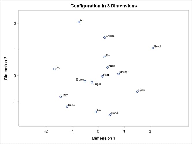
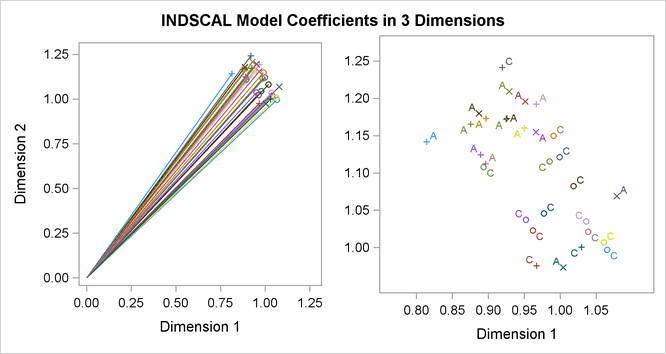
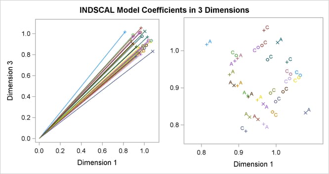
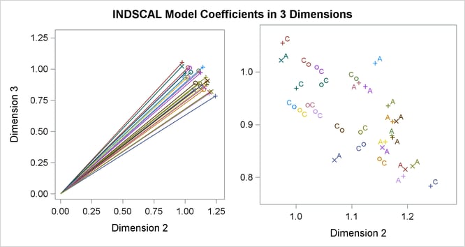
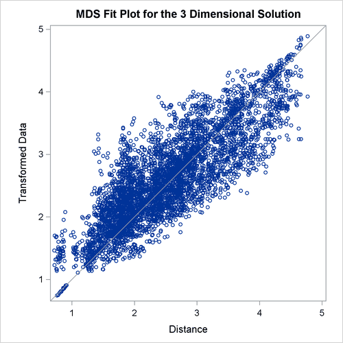
Often the output of greatest interest in an MDS analysis is the graphical output. The first plots show two-dimensional view of the three-dimensional configuration. Next, the coefficients are plotted. The last plot is the fit plot.
In the fit plot, the transformed data are plotted on the vertical axis, and the distances from the model are plotted on the horizontal axis. If the model fits perfectly, all points lie on a diagonal line from lower left to upper right. The vertical departure of each point from this diagonal line represents the residual of the corresponding observation.
The configuration has a tripodal shape with Body at the apex. The three legs of the tripod can be distinguished in the plot of dimension 2 by dimension 1, which shows three
distinct clusters with Body in the center. Dimension 1 separates head parts from arm and leg parts. Dimension 2 separates arm parts from leg parts. The
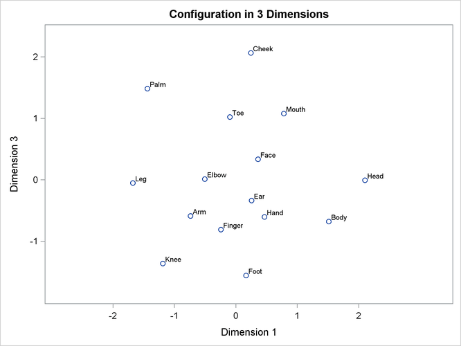
plot of dimension 3 by dimension 1 shows the tripod from the side. Dimension 3 distinguishes the more inclusive body parts
(at the top) from the less inclusive body parts (at the bottom).
The plots of dimension coefficients show that children differ from adults primarily in the emphasis given to dimension 2. Children give about the same weight (approximately 1) to each dimension. Adults are much more variable than children, but all have coefficients less than 1.0 for dimension 2, with an average of about 0.7. Referring back to the configuration plot, you can see that adults consider arm parts to be more similar to leg parts than children do. Many adults also give a high weight to dimension 1, indicating that they consider head parts to be more dissimilar from arm and leg parts than children do. Dimension 3 shows considerable variability for both children and adults.