The MCMC Procedure
-
Overview

-
Getting Started
-
Syntax
-
DetailsHow PROC MCMC WorksBlocking of ParametersSampling MethodsTuning the Proposal DistributionDirect SamplingConjugate SamplingInitial Values of the Markov ChainsAssignments of ParametersStandard DistributionsUsage of Multivariate DistributionsSpecifying a New DistributionUsing Density Functions in the Programming StatementsTruncation and CensoringSome Useful SAS FunctionsMatrix Functions in PROC MCMCCreate Design MatrixModeling Joint LikelihoodRegenerating Diagnostics PlotsCaterpillar PlotAutocall Macros for PostprocessingGamma and Inverse-Gamma DistributionsPosterior Predictive DistributionHandling of Missing DataFunctions of Random-Effects ParametersFloating Point Errors and OverflowsHandling Error MessagesComputational ResourcesDisplayed OutputODS Table NamesODS Graphics
-
ExamplesSimulating Samples From a Known DensityBox-Cox TransformationLogistic Regression Model with a Diffuse PriorLogistic Regression Model with Jeffreys’ PriorPoisson RegressionNonlinear Poisson Regression ModelsLogistic Regression Random-Effects ModelNonlinear Poisson Regression Multilevel Random-Effects ModelMultivariate Normal Random-Effects ModelMissing at Random AnalysisNonignorably Missing Data (MNAR) AnalysisChange Point ModelsExponential and Weibull Survival AnalysisTime Independent Cox ModelTime Dependent Cox ModelPiecewise Exponential Frailty ModelNormal Regression with Interval CensoringConstrained AnalysisImplement a New Sampling AlgorithmUsing a Transformation to Improve MixingGelman-Rubin Diagnostics
- References
Example 55.1 Simulating Samples From a Known Density
This example illustrates how you can obtain random samples from a known function. The target distributions are the normal distribution (a standard distribution) and a mixture of the normal distributions (a nonstandard distribution). For more information, see the sections Standard Distributions and Specifying a New Distribution). This example also shows how you can use PROC MCMC to estimate an integral (area under a curve). Monte Carlo simulation is data-independent; hence, you do not need an input data set from which to draw random samples from the desired distribution.
Sampling from a Normal Density
When you run a simulation without an input data set, the posterior distribution is the same as the prior distribution. Hence, if you want to generate samples from a distribution, you declare the distribution in the PRIOR statement and set the likelihood function to a constant. Although there is no contribution from any data set variable to the likelihood calculation, you still must specify a data set and the MODEL statement needs a distribution. You can input an empty data set and use the GENERAL function to provide a flat likelihood. The following statements generate 10,000 samples from a standard normal distribution:
title 'Simulating Samples from a Normal Density';
data x;
run;

ods graphics on;
proc mcmc data=x outpost=simout seed=23 nmc=10000
     statistics=(summary interval) diagnostics=none;
   ods exclude nobs;
   parm alpha 0;
   prior alpha ~ normal(0, sd=1);
   model general(0);
run;
The ODS GRAPHICS ON statement enables ODS Graphics. The PROC MCMC statement specifies the input and output data sets, a random number seed, and the size of the simulation sample. The STATISTICS= option displays only the summary and interval statistics. The ODS EXCLUDE statement excludes the display of the NObs table. PROC MCMC draws independent samples from the normal distribution directly (see Output 55.1.1). Therefore, the simulation does not require any tuning, and PROC MCMC omits the default burn-in phrase.
Output 55.1.1: Parameters Information
| Simulating Samples from a Normal Density |
| Parameters | ||||
|---|---|---|---|---|
| Block | Parameter | Sampling Method |
Initial Value |
Prior Distribution |
| 1 | alpha | Direct | 0 | normal(0, sd=1) |
The summary statistics (Output 55.1.2) are what you would expect from a standard normal distribution.
Output 55.1.2: MCMC Summary and Interval Statistics from a Normal Target Distribution
| Simulating Samples from a Normal Density |
| Posterior Summaries | ||||||
|---|---|---|---|---|---|---|
| Parameter | N | Mean | Standard Deviation |
Percentiles | ||
| 25% | 50% | 75% | ||||
| alpha | 10000 | 0.00195 | 0.9949 | -0.6544 | 0.00965 | 0.6709 |
| Posterior Intervals | |||||
|---|---|---|---|---|---|
| Parameter | Alpha | Equal-Tail Interval | HPD Interval | ||
| alpha | 0.050 | -1.9485 | 1.9507 | -1.9664 | 1.9302 |
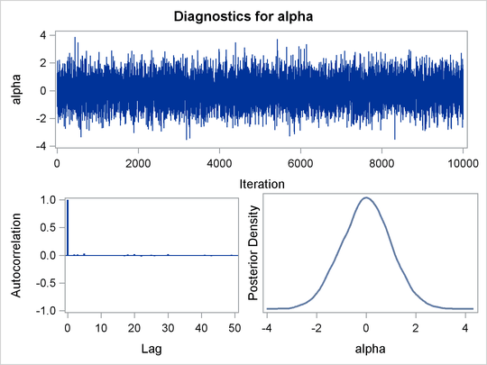
The trace plot (Output 55.1.3) shows perfect mixing with no autocorrelation in the lag plot. This is expected because these are independent draws.
Output 55.1.3: Diagnostics Plots for ![]()
You can overlay the estimated kernel density with the true density to visually compare the densities, as displayed in Output 55.1.4. To create the kernel comparison plot, you first call PROC KDE (see Chapter 48: The KDE Procedure,) to obtain a kernel density estimate of the posterior density on alpha. Then you evaluate a grid of alpha values on a normal density. The following statements evaluate kernel density and compute the corresponding normal density:
proc kde data=simout;
   ods exclude inputs controls;
   univar alpha /out=sample;
run;

data den;
   set sample;
   alpha = value;
   true  = pdf('normal', alpha, 0, 1);
   keep alpha density true;
run;
Next you plot the two curves on top of each other by using PROC SGPLOT (see Chapter 21: Statistical Graphics Using ODS,) as follows:
proc sgplot data=den;
   yaxis label="Density";
   series y=density x=alpha / legendlabel = "MCMC Kernel";
   series y=true x=alpha / legendlabel = "True Density";
   discretelegend;
run;
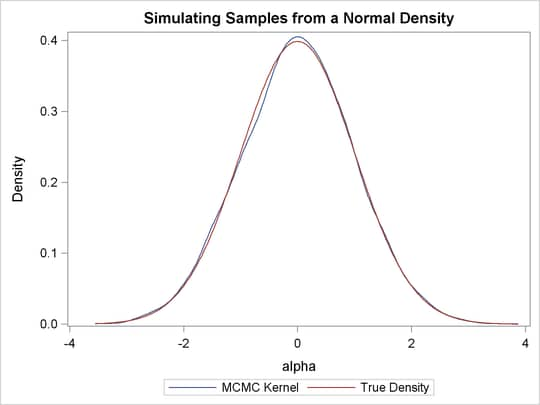
Output 55.1.4 shows the result. You can see that the kernel estimate and the true density are very similar to each other.
Output 55.1.4: Estimated Density versus the True Density
Density Visualization Macro
In programs that do not involve any data set variables, PROC MCMC samples directly from the (joint) prior distributions of the parameters. The modification makes the sampling from a known distribution more efficient and more precise. For example, you can write simple programs, such as the following macro, to understand different aspects of a prior distribution of interest, such as its moments, intervals, shape, spread, and so on:
%macro density(dist=, seed=0);
   %let savenote = %sysfunc(getoption(notes));
   options nonotes;
   title "&dist distribution.";
   data _a;
   run;

   ods select densitypanel postsummaries postintervals;
   proc mcmc data=_a nmc=10000 diag=none nologdist
      plots=density seed=&seed;
      parms alpha;
      prior alpha ~ &dist;
      model general(0);
   run;

   proc datasets nolist;
      delete _a;
   run;
   options &savenote;
%mend;

%density(dist=beta(4, 12), seed=1);
The macro %density creates an empty data set, invokes PROC MCMC, draws 10,000 samples from a beta(4, 12) distribution, displays summary and
interval statistics, and generates a kernel density plot. Summary and interval statistics from the beta distribution are displayed
in Output 55.1.5.
Output 55.1.5: Beta Distribution Statistics
| beta(4, 12) distribution. |
| Posterior Summaries | ||||||
|---|---|---|---|---|---|---|
| Parameter | N | Mean | Standard Deviation |
Percentiles | ||
| 25% | 50% | 75% | ||||
| alpha | 10000 | 0.2494 | 0.1039 | 0.1731 | 0.2397 | 0.3148 |
| Posterior Intervals | |||||
|---|---|---|---|---|---|
| Parameter | Alpha | Equal-Tail Interval | HPD Interval | ||
| alpha | 0.050 | 0.0775 | 0.4800 | 0.0657 | 0.4590 |
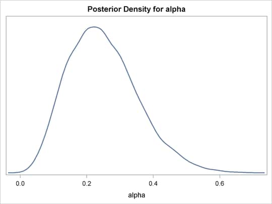
The distribution is displayed in Output 55.1.6.
Output 55.1.6: Density Plot
Calculation of Integrals
One advantage of MCMC methods is to estimate any integral under the curve of a target distribution. This can be done fairly easily using the MCMC procedure. Suppose you are interested in estimating the following cumulative probability:
|
|
To estimate this integral, PROC MCMC draws samples from the distribution and counts the portion of the simulated values that fall within the desired range of [0, 1.3]. This becomes a Monte Carlo estimate of the integral. The following statements simulate samples from a standard normal distribution and estimate the integral:
proc mcmc data=x outpost=simout seed=23 nmc=10000 nologdist
   monitor=(int) statistics=(summary) diagnostics=none;
   ods select postsummaries;
   parm alpha 0;
   prior alpha ~ normal(0, sd=1);
   int = (0 <= alpha <= 1.3);
   model general(0);
run;
The ODS SELECT statement displays the posterior summary statistics table. The MONITOR= option outputs analysis on the variable int (the integral estimate). The STATISTICS= option computes the summary statistics. The NOLOGDIST option omits the calculation of the log of the prior distribution at each iteration, shortening the simulation time[6]. The INT assignment statement sets int to be 1 if the simulated alpha value falls between 0 and 1.3, and 0 otherwise. PROC MCMC supports the usage of the IF-ELSE logical control if you need to
account for more complex conditions. Output 55.1.7 displays the estimated integral value:
Output 55.1.7: Monte Carlo Integral from a Normal Distribution
| beta(4, 12) distribution. |
| Posterior Summaries | ||||||
|---|---|---|---|---|---|---|
| Parameter | N | Mean | Standard Deviation |
Percentiles | ||
| 25% | 50% | 75% | ||||
| int | 10000 | 0.4079 | 0.4915 | 0 | 0 | 1.0000 |
In this simulation, 4079 samples fall between 0 and 1.3, making the expected probability 0.4079. In this example, you can verify the actual cumulative probability by calling the CDF function in the DATA step:
data _null_;
   int = cdf("normal", 1.3, 0, 1) - cdf("normal", 0, 0, 1);
   put int=;
run;
The value is 0.4032.
Sampling from a Mixture of Normal Densities
Suppose you are interested in generating samples from a three-component mixture of normal distributions, with the density specified as follows:
|
|
The distribution is not one of the standard distributions that PROC MCMC supports. Hence you need to construct the density function and supply it to the procedure. The following statements generate random samples from this mixture density:
title 'Simulating Samples from a Mixture of Normal Densities';
data x;
run;

proc mcmc data=x outpost=simout seed=1234 nmc=30000;
   ods select TADpanel;
   parm alpha 0.3;
   lp = logpdf('normalmix', alpha, 3, 0.3, 0.4, 0.3, -3, 2, 10, 2, 1, 4);
   prior alpha  ~ general(lp);
   model general(0);
run;
The ODS SELECT statement displays the diagnostic plots. All other tables, such as the NObs tables, are excluded. The PROC MCMC statement uses the input data set X, saves output to the Simout data set, sets a random number seed, and draws 30,000 samples.
The LP assignment statement evaluates the log density of alpha at the mixture density, using the SAS function LOGPDF. The number 3 after alpha in the LOGPDF function indicates that the density is a three-component normal mixture. The following three numbers, 0.3,
0.4, and 0.3, are the weights in the mixture; –3, 2, and 10 are the means; 2, 1, and 4 are the standard deviations. The PRIOR statement assigns this log density function to alpha as its prior. Note that the GENERAL function interprets the density on the log scale, and not the original scale–you must use the LOGPDF function, not the PDF
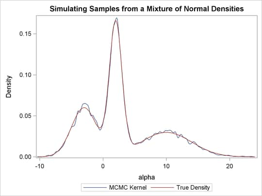
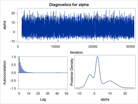
function. Output 55.1.8 displays the results. The kernel density clearly shows three modes.
Output 55.1.8: Plots of Posterior Samples from a Mixture Normal Distribution
Using the following set of statements similar to the previous example, you can overlay the estimated kernel density with the true density. The comparison is shown in Output 55.1.9.
proc kde data=simout;
   ods exclude inputs controls;
   univar alpha /out=sample;
run;

data den;
   set sample;
   alpha = value;
   true  = pdf('normalmix', alpha, 3, 0.3, 0.4, 0.3, -3, 2, 10, 2, 1, 4);
   keep alpha density true;
run;

proc sgplot data=den;
   yaxis label="Density";
   series y=density x=alpha / legendlabel = "MCMC Kernel";
   series y=true x=alpha / legendlabel = "True Density";
   discretelegend;
run;
Output 55.1.9: Estimated Density versus the True Density