The MCMC Procedure

Standard Distributions

Univariate Distributions
Multivariate Distributions

The section Univariate Distributions (Table 55.7 through Table 55.34) lists all univariate distributions that PROC MCMC recognizes. The section Multivariate Distributions (Table 55.35 through Table 55.39) lists all multivariate distributions that PROC MCMC recognizes. With the exception of the multinomial distribution, all these distributions can be used in the MODEL, PRIOR, and HYPERPRIOR statements. The multinomial distribution is supported only in the MODEL statement. The RANDOM statement supports a limited number of distributions; see Table 55.4 for the complete list.

See the section Using Density Functions in the Programming Statements for information about how to use distributions in the programming statements. To specify an arbitrary distribution, you can use the GENERAL and DGENERAL functions. See the section Specifying a New Distribution for more details. See the section Truncation and Censoring for tips about how to work with truncated distributions and censoring data.

Univariate Distributions

Table 55.7: Beta Distribution

PROC specification	beta(a, b)
Density	$\frac{\Gamma (a+b)}{\Gamma (a) \Gamma (b)} \theta ^{a-1} (1-\theta )^{b-1}$
Parameter restriction	,
Range	$\left\{ \begin{array}{ll} \left[ 0, 1 \right] & \mbox{when } a = 1, b = 1 \\ \left[ 0, 1 \right) & \mbox{when } a = 1, b \neq 1 \\ \left( 0, 1 \right] & \mbox{when } a \neq 1, b = 1 \\ \left( 0, 1 \right) & \mbox{otherwise} \end{array} \right.$
Mean	$\frac{a}{a+b}$
Variance	$\frac{ab}{(a+b)^2(a+b+1)}$
Mode	$\left\{ \begin{array}{ll} \frac{a-1}{a+b-2} & a > 1, b > 1 \\ 0 \mbox{ and } 1 & a < 1, b < 1 \\ 0 & \left\{ \begin{array}{l} a < 1, b \geq 1 \\ a = 1, b > 1 \\ \end{array} \right. \\ 1 & \left\{ \begin{array}{l} a \geq 1, b < 1 \\ a > 1, b = 1 \\ \end{array} \right. \\ \mbox{does not exist uniquely} & a = b = 1 \end{array} \right.$
Random number	If $\min (a,b) > 1$ , see (Cheng, 1978); if $\max (a, b) < 1$ , see (Atkinson and Whittaker, 1976) and (Atkinson, 1979); if $\min (a, b) < 1$ and $\max (a, b) > 1$ , see (Cheng, 1978); if or , use the inversion method; if , use a uniform random number generator.

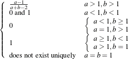
Table 55.8: Binary Distribution

PROC specification	binary(p)
Density	$p^\theta (1-p)^{1-\theta }$
Parameter restriction	$0 \leq p \leq 1$
Range	$\left\{ \begin{array}{ll} \{ 0\} & \mbox{when } p = 0 \\ \{ 1\} & \mbox{when } p = 1 \\ \{ 0, 1 \} & \mbox{otherwise} \end{array} \right.$
Mean	round
Variance
Mode	$\left\{ \begin{array}{ll} \{ 1\} & \mbox{when } p = 1 \\ \{ 0\} & \mbox{otherwise} \end{array} \right.$
Random number	Generate $u \sim \mbox{uniform}(0, 1)$ . If $u \leq p$ , $\theta = 1$ ; else, $\theta = 0.$

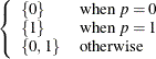
Table 55.9: Binomial Distribution

PROC specification	binomial(n, p)
Density	$\left(\begin{array}{l} n \\ \theta \end{array} \right) p^\theta (1-p)^{n-\theta }$
Parameter restriction	$n = {0, 1, 2, \cdots } \; 0 \leq p \leq 1$
Range	$\theta \in \{ 0, \cdots , n \}$
Mean	$\lfloor np \rfloor$
Variance
Mode	$\lfloor (n+1)p \rfloor$

Table 55.10: Cauchy Distribution

PROC specification	cauchy(a, b)
Density	$\frac{1}{\pi } \left( \frac{b}{b^2 + (\theta -a)^2} \right)$
Parameter restriction
Range	$\theta \in (-\infty , \infty )$
Mean	Does not exist.
Variance	Does not exist.
Mode	a
Random number	Generate $u_1, u_2 \sim \mbox{uniform}(0, 1)$ ; let . Repeat the procedure until . is a draw from the standard Cauchy, and $\theta = a+by$ (Ripley, 1987).

Table 55.11: $\chi ^2$ Distribution

PROC specification	chisq( $\nu$ )
Density	$\frac{1}{\Gamma (\nu /2) 2^{\nu /2}} \theta ^{(\nu /2)-1} e^{-\theta /2}$
Parameter restriction	$\nu > 0$
Range	$\theta \in [0, \infty )$ if $\nu = 2$ ; $(0, \infty )$ otherwise.
Mean	$\nu$
Variance	$2\nu$
Mode	$\nu - 2$ if $\nu \geq 2$ ; does not exist otherwise.
Random number	$\chi ^2$ is a special case of the gamma distribution: $\theta \sim \mbox{gamma}(\nu /2, \mbox{scale=} 2)$ is a draw from the $\chi ^2$ distribution.

Table 55.12: Exponential $\chi ^2$ Distribution

PROC specification	expchisq( $\nu$ )
Density	$\frac{1}{\Gamma ( \nu /2) 2^{\nu /2}} \exp ( \theta )^{\nu /2}\exp ( -\exp ( \theta ) /2 )$
Parameter restriction	$\nu > 0$
Range	$\theta \in (-\infty , \infty )$
Mode	$\log (\nu )$
Random number	Generate $x_1 \sim \chi ^2(\nu )$ , and $\theta = \log (x_1)$ is a draw from the exponential $\chi ^2$ distribution.
Relationship to the $\chi ^2$ distribution	$\theta \sim \chi ^2(\nu ) \Leftrightarrow \log (\theta ) \sim \exp \chi ^2(\nu )$

Table 55.13: Exponential Exponential Distribution

PROC specification	expexpon(`scale =` b )	expexpon(`iscale =` $\beta$ )
Density	$\frac{1}{b}\exp ( \theta ) \exp (-\exp (\theta ) /b)$	$\beta \exp (\theta ) \exp (-\exp ( \theta ) \cdot \beta )$
Parameter restriction		$\beta > 0$
Range	$\theta \in (-\infty , \infty )$	Same
Mode	$\log (b)$	$\log (1/\beta )$
Random number	Generate $x_1 \sim \mbox{expon}(\mbox{scale=} b)$ , and $\theta = \log (x_1)$ is a draw from the exponential exponential distribution. Note that an exponential exponential distribution is not the same as the double exponential distribution.
Relationship to the exponential distribution	$\theta \sim \mbox{expon}(b) \Leftrightarrow \log (\theta ) \sim \mbox{expExpon}(b)$

Table 55.14: Exponential Gamma Distribution

PROC specification	expgamma(a, `scale =` b )	expgamma(a, `iscale =` $\beta$ )
Density	$\frac{1}{b^{a}\Gamma (a)} e^{a \theta } \exp (-e^{\theta } /b )$	$\frac{\beta ^{a}}{\Gamma (a) } e^{a \theta } \exp ( - e^{\theta } \cdot \beta )$
Parameter restriction		$a > 0, \beta > 0$
Range	$\theta \in (-\infty , \infty )$	Same
Mode	$\log (ab)$	$\log (a/\beta )$
Random number	Generate $x_1 \sim \mbox{gamma}(a, \mbox{scale} = b)$ , and $\theta = \log (x_1)$ is a draw from the exponential gamma distribution.
Relationship to the $\Gamma$ distribution	$\theta \sim \mbox{gamma}(a, b) \Leftrightarrow \log (\theta ) \sim \mbox{expGamma}(a, b)$

Table 55.15: Exponential Inverse $\chi ^2$ Distribution

PROC specification	expichisq( $\nu$ )
Density	$\frac{1}{\Gamma ( \frac{\nu }{2}) 2^{\nu /2}}\exp ( -\nu \theta / 2 ) \exp ( -1/(2\exp ( \theta ) ))$
Parameter restriction	$\nu > 0$
Range	$\theta \in (-\infty , \infty )$
Mode	$-\log (\nu )$
Random number	Generate $x_1 \sim i\chi ^2(\nu )$ , and $\theta = \log (x_1)$ is a draw from the exponential inverse $\chi ^2$ distribution.
Relationship to the $i\chi ^2$ distribution	$\theta \sim i\chi ^2(\nu ) \Leftrightarrow \log (\theta ) \sim \exp i\chi ^2(\nu )$

Table 55.16: Exponential Inverse-Gamma Distribution

PROC specification	expigamma(a, `scale =` b )	expigamma(a, `iscale =` $\beta$ )
Density	$\frac{b^{a}}{\Gamma (a) } \exp ( -\alpha \theta ) \exp ( -b/\exp ( \theta ) )$	$\frac{1}{\beta ^{\alpha }\Gamma ( a) } \exp ( -\alpha \theta ) \exp ( -\frac{1}{ \beta \exp ( \theta ) })$
Parameter restriction		$a > 0, \beta > 0$
Range	$\theta \in (-\infty , \infty )$	Same
Mode	$-\log (a/b)$	$-\log (a\beta )$
Random number	Generate $x_1 \sim \mbox{igamma}(a, \mbox{scale} = b)$ , and $\theta = \log (x_1)$ is a draw from the exponential inverse-gamma distribution.
Relationship to the $i\Gamma$ distribution	$\theta \sim \mbox{igamma}(a, b) \Leftrightarrow \log (\theta ) \sim \mbox{eigamma}(a, b)$

Table 55.17: Exponential Scaled Inverse $\chi ^2$ Distribution

PROC specification	expsichisq( $\nu$ , s)
Density	$\frac{ (\frac{\nu }{2}) ^{\nu /2}}{ \Gamma ( \frac{\nu }{2}) }s^{\nu }\exp (-\nu \theta /2) \exp ( -\nu s^{2}/(2\exp (\theta )))$
Parameter restriction	$\nu > 0, s > 0$
Range	$\theta \in (-\infty , \infty )$
Mode	$\log (s^2)$
Random number	Generate $x_1 \sim si\chi ^2(\nu , s)$ , and $\theta = \log (x_1)$ is a draw from the exponential scaled inverse $\chi ^2$ distribution.
Relationship to the $si\chi ^2$ distribution	$\theta \sim si\chi ^2(\nu , s) \Leftrightarrow \log (\theta ) \sim \exp si\chi ^2(\nu , s)$

Table 55.18: Exponential Distribution

PROC specification	expon(`scale =` b )	expon(`iscale =` $\beta$ )
Density	$\frac{1}{b} e^{-\theta /b}$	$\beta e^{-\beta \theta }$
Parameter restriction		$\beta > 0$
Range	$\theta \in [0, \infty )$	Same
Mean	b	$1/\beta$
Variance		$1/\beta ^2$
Mode	0	0
Random number	The exponential distribution is a special case of the gamma distribution: $\theta \sim \mbox{gamma}(1, \mbox{scale} = b)$ is a draw from the exponential distribution.

Table 55.19: Gamma Distribution

PROC specification	gamma(a, `scale =` b )	gamma(a, `iscale =` $\beta$ )
Density	$\frac{1}{b^ a\Gamma (a)} \theta ^{a-1} e^{-\theta /b}$	$\frac{\beta ^ a}{\Gamma (a)} \theta ^{a-1} e^{-\beta \theta }$
Parameter restriction		$a > 0, \beta > 0$
Range	$\theta \in [0, \infty )$ if $a=1; (0, \infty )$ otherwise.	Same
Mean	ab	$a/\beta$
Variance		$a/\beta ^2$
Mode	if $a \geq 1$	$(a-1)/\beta$ if $a \geq 1$
Random number	See (McGrath and Irving, 1973).

Table 55.20: Geometric Distribution

PROC specification

geo(p)

Density ^[a]

$p(1-p)^\theta$

Parameter restriction

$0 < p \leq 1$

Range

$\theta \in \left\{ \begin{array}{ll} \{ 0, 1, 2, \ldots \} & 0 < p < 1 \\ \{ 0\} & p = 1 \\ \end{array} \right.$

Mean

round( $\frac{1-p}{p}$ )

Variance

$\frac{1-p}{p^2}$

Mode

Random number

Based on samples obtained from a Bernoulli distribution with probability p until the first success.

^[a]The random variable $\theta$ is the total number of failures in an experiment before the first success. This density function is not to be confused with another popular formulation, $p (1-p)^{\theta -1}$ , which counts the total number of trials until the first success.

Table 55.21: Inverse $\chi ^2$ Distribution

PROC specification	ichisq( $\nu$ )
Density	$\frac{1}{\Gamma (\nu /2) 2^{\nu /2}} \theta ^{-(\nu /2+1)} e^{-1/(2\theta )}$
Parameter restriction	$\nu > 0$
Range	$\theta \in (0, \infty )$
Mean	$\frac{1}{\nu -2}$ if $\nu > 2$
Variance	$\frac{2}{(\nu -2)^2(\nu -4)}$ if $\nu > 4$
Mode	$\frac{1}{\nu + 2}$
Random number	Inverse $\chi ^2$ is a special case of the inverse-gamma distribution: $\theta \sim \mbox{igamma}( \nu /2, \mbox{iscale} = 2)$ is a draw from the inverse $\chi ^2$ distribution.

Table 55.22: Inverse-Gamma Distribution

PROC specification	igamma(a, `scale =` b )	igamma(a, `iscale =` $\beta$ )
Density	$\frac{b^ a}{\Gamma (a)} \theta ^{-(a+1)} e^{-b/\theta }$	$\frac{1}{\beta ^ a \Gamma (a)} \theta ^{-(a+1)} e^{-1/\beta \theta }$
Parameter restriction		$a > 0, \beta > 0$
Range	$\theta \in (0, \infty )$	Same
Mean	$\frac{b}{a-1}$ if	$\frac{1}{\beta (a-1)}$ if
Variance	$\frac{b^2}{(a-1)^2(a-2)}$	$\frac{1}{\beta ^2(a-1)^2(a-2)}$
Mode	$\frac{b}{a+1}$	$\frac{1}{\beta (a+1)}$
Random number	Generate $x_1 \sim \mbox{gamma}(a, \mbox{scale} = b)$ , and $\theta = 1/x_1$ is a draw from the $\mbox{igamma}(a, \mbox{iscale} = b)$ distribution.
Relationship to the gamma distribution	$\theta \sim \mbox{gamma}(a, \mbox{iscale} = b) \Leftrightarrow 1/\theta \sim \mbox{igamma}(a, \mbox{scale} = b)$

Table 55.23: Laplace (Double Exponential) Distribution

PROC specification	laplace(a, `scale =` b)	laplace(a, `iscale =` $\beta$ )
Density	$\frac{1}{2b} e^{-\|\theta -a\|/b}$	$\frac{\beta }{2} e^{-\beta \|\theta -a\|}$
Parameter restriction		$\beta > 0$
Range	$\theta \in (-\infty , \infty )$	Same
Mean	a	a
Variance		$2 / \beta ^2$
Mode	a	a
Random number	Inverse CDF. $F(\theta ) = \left\{ \begin{array}{ll} \frac{1}{2} \exp \left( -\frac{a-\theta }{b}\right) & \theta < a \\ 1 - \frac{1}{2} \exp \left( -\frac{\theta - a}{b}\right) & \theta \geq a \end{array} \right. .$ Generate $u_1, u_2 \sim \mbox{uniform}(0, 1)$ . If $u_1 < 0.5, \theta = a + b\log (u_2);$ else $\theta = a - b \log (u_2)$ . $\theta$ is a draw from the Laplace distribution.

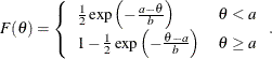
Table 55.24: Logistic Distribution

PROC specification	logistic(a, b)
Density	$\frac{\exp \left(-\frac{\theta -a}{b} \right)}{b \left(1+\exp \left( -\frac{\theta -a}{b} \right) \right)^2}$
Parameter restriction
Range	$\theta \in (-\infty , \infty )$
Mean	a
Variance	$\frac{\pi ^2 b^2}{3}$
Mode	a
Random number	Inverse CDF method with $F(\theta ) = \left(1 + \exp (-\frac{\theta - a}{b}) \right)^{-1}$ . Generate $u \sim \mbox{uniform}(0,1)$ , and $\theta = a - b\log (1/u-1)$ is a draw from the logistic distribution.

Table 55.25: Lognormal Distribution

PROC specification	lognormal( $\mu$ , `sd =` s)	lognormal( $\mu$ , `var =` v)	lognormal( $\mu$ , `prec =` $\tau$ )
Density	$\frac{1}{\theta s\sqrt {2\pi }} \exp \left( - \frac{(\log {\theta } - \mu )^2}{2s^2} \right)$	$\frac{1}{\theta \sqrt {2\pi v}} \exp \left( - \frac{(\log {\theta } - \mu )^2}{2v} \right)$	$\frac{1}{\theta } \sqrt {\frac{\tau }{2\pi }} \exp \left( - \frac{\tau (\log {\theta } - \mu )^2}{2} \right)$
Parameter restriction			$\tau > 0$
Range	$\theta \in (0, \infty )$	Same	Same
Mean	$\exp (\mu + s^2/2)$	$\exp (\mu + v/2)$	$\exp (\mu + 1/(2\tau ))$
Variance	$\begin{array}{l} \exp {(2(\mu +s^2))} \\ - \exp {(2\mu +s^2)} \end{array}$	$\begin{array}{l} \exp {(2(\mu +v))} \\ - \exp {(2\mu +v)} \end{array}$	$\begin{array}{l} \exp {(2(\mu +1/\tau ))} \\ - \exp {(2\mu +1/\tau )} \end{array}$
Mode	$\exp (\mu - s^2)$	$\exp (\mu - v)$	$\exp (\mu - 1/\tau )$
Random number	Generate $x_1 \sim \mbox{normal}(0, 1)$ , and $\theta = \exp (\mu + sx_1)$ is a draw from the lognormal distribution.

Table 55.26: Negative Binomial Distribution

PROC specification	negbin(n, p)
Density	$\left( \begin{array}{c} \theta +n-1 \\ n - 1 \end{array} \right) p^ n (1-p)^\theta$
Parameter restriction	$n = {1, 2, \cdots }, \mbox{and} 0 < p \leq 1$
Range	$\theta \in \left\{ \begin{array}{ll} \{ 0, 1, 2, \ldots \} & 0 < p < 1 \\ \{ 0\} & p = 1 \\ \end{array} \right.$
Mean	round $\left(\frac{n(1-p)}{p}\right)$
Variance	$\frac{n(1-p)}{p^2}$
Mode	$\left\{ \begin{array}{ll} 0 & n = 1 \\ \mbox{round} \left( \frac{(n-1)(1-p)}{p} \right) & n > 1 \end{array} \right.$
Random number	Generate $x_1 \sim \mbox{gamma}(n, 1)$ , and $\theta \sim \mbox{Poisson}(x_1 \cdot (1-p) / p)$ (Fishman, 1996).

Table 55.27: Normal Distribution

PROC specification	normal( $\mu$ , `sd =` s)	normal( $\mu$ , `var =` v)	normal( $\mu$ , `prec =` $\tau$ )
Density	$\frac{1}{s\sqrt {2\pi }} \exp \left( - \frac{(\theta - \mu )^2}{2s^2}\right)$	$\frac{1}{\sqrt {2\pi v}} \exp \left( - \frac{(\theta - \mu )^2}{2v}\right)$	$\sqrt {\frac{\tau }{2\pi }} \exp \left( - \frac{\tau (\theta - \mu )^2}{2}\right)$
Parameter restriction			$\tau > 0$
Range	$\theta \in (-\infty , \infty )$	Same	Same
Mean	$\mu$	Same	Same
Variance		v	$1/\tau$
Mode	$\mu$	Same	Same

Table 55.28: Pareto Distribution

PROC specification	pareto(a, b)
Density	$\frac{a}{b} \left( \frac{b}{\theta } \right)^{a+1}$
Parameter restriction
Range	$\theta \in [b, \infty )$
Mean	$\frac{ab}{a-1}$ if
Variance	$\frac{b^2a}{(a-1)^2(a-2)}$ if
Mode	b
Random number	Inverse CDF method with $F(\theta ) = 1 - (b/\theta )^ a$ . Generate $u \sim \mbox{uniform}(0,1)$ , and $\theta = \frac{b}{u^{1/a}}$ is a draw from the Pareto distribution.
Useful transformation	$x = 1/\theta$ is Beta(a, 1)I{}.

Table 55.29: Poisson Distribution

PROC specification	poisson( $\lambda$ )
Density	$\frac{\lambda ^\theta }{\theta !}\exp (-\lambda )$
Parameter restriction	$\lambda \geq 0$
Range	$\theta \in \left\{ \begin{array}{ll} \{ 0, 1, \ldots \} & \mbox{if} \; \lambda > 0 \\ \{ 0 \} & \mbox{if} \; \lambda = 0 \\ \end{array} \right.$
Mean	$\lambda$
Variance	$\lambda$ , if $\lambda > 0$
Mode	round $(\lambda )$

Table 55.30: Scaled Inverse $\chi ^2$ Distribution

PROC specification	sichisq( $\nu , s^2$ )
Density	$\frac{(s^2 \nu /2)^{\nu /2}}{\Gamma (\nu /2)} \theta ^{-(\nu /2+1)} e^{-\nu s^2/(2\theta )}$
Parameter restriction	$\nu > 0, s > 0$
Range	$\theta \in (0, \infty )$
Mean	$\frac{\nu }{\nu -2} s^2$ if $\nu > 2$
Variance	$\frac{2\nu ^2}{(\nu -2)^2(\nu -4)} s^4$ if $\nu > 4$
Mode	$\frac{\nu }{\nu + 2} s^2$
Random number	Scaled inverse $\chi ^2$ is a special case of the inverse-gamma distribution: $\theta \sim \mbox{igamma}( \nu /2, \mbox{scale} = (\nu s^2)/2)$ is a draw from the scaled inverse $\chi ^2$ distribution.

Table 55.31: t Distribution

PROC specification	t( $\mu$ , `sd =` s, $\nu$ )	t( $\mu$ , `var =` v, $\nu$ )	t( $\mu$ , `prec =` $\tau$ , $\nu$ )
Density	$\frac{\Gamma ( \frac{\nu +1}{2})}{\Gamma ( \frac{\nu }{2} ) s \sqrt {\nu \pi }} ( 1 + \frac{(\theta -\mu )^2}{\nu s^2}) ^{-\frac{\nu +1}{2}}$	$\frac{\Gamma ( \frac{\nu +1}{2} )}{\Gamma ( \frac{\nu }{2} ) \sqrt {\nu \pi v}} ( 1 + \frac{ (\theta -\mu )^2 }{\nu v} )^{-\frac{\nu +1}{2}}$	$\frac{\Gamma ( \frac{\nu +1}{2}) \sqrt {\tau }}{\Gamma ( \frac{\nu }{2} ) \sqrt {\nu \pi }} ( 1 + \frac{\tau (\theta -\mu )^2}{\nu }) ^{-\frac{\nu +1}{2}}$
Parm restriction	, $\nu > 0$	, $\nu > 0$	$\tau > 0$ , $\nu > 0$
Range	$\theta \in (-\infty , \infty )$	Same	Same
Mean	$\mu$ if $\nu > 1$	Same	Same
Variance	$\frac{\nu }{\nu -2} s^2$ if $\nu > 2$	$\frac{\nu }{\nu -2} v$ if $\nu > 2$	$\frac{\nu }{\nu -2} \frac{1}{\tau }$ if $\nu > 2$
Mode	$\mu$	Same	Same
Random number	$x_1 \sim \mbox{normal}(0, 1), x_2 \sim \chi ^2(d), \mbox{ and }\theta = m + \sigma x_1 \sqrt {d/x_2}$ is a draw from the t distribution.

Table 55.32: Uniform Distribution

PROC specification	uniform(a, b)
Density	$\left\{ \begin{array}{ll} \frac{1}{a-b} & \mbox{if} \; a>b \\ \frac{1}{b-a} & \mbox{if} \; b>a \\ 1 & \mbox{if} \; a=b \end{array} \right.$
Parameter restriction	none
Range	$\theta \in [a, b]$
Mean	$\frac{a+b}{2}$
Variance	$\frac{\|b-a\|^2}{12}$
Mode	Does not exist
Random number	Mersenne Twister (Matsumoto and Kurita, 1992, 1994; Matsumoto and Nishimura, 1998)

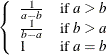
Table 55.33: Wald Distribution

PROC specification	wald( $\mu$ , $\lambda$ )
Density	$\sqrt {\frac{\lambda }{2\pi \theta ^3}} \exp \left( \frac{-\lambda (\theta -\mu )^2}{2\mu ^2\theta }\right)$
Parameter restriction	$\mu > 0, \lambda > 0$
Range	$\theta \in (0, \infty )$
Mean	$\mu$
Variance	$\mu ^3 / \lambda$
Mode	$\mu \left[ \left( 1 + \frac{9\mu ^2}{4\lambda ^2}\right)^{1/2} - \frac{3\mu }{2\lambda } \right]$
Random number	Generate $\nu _0 \sim \chi ^2_{(1)}$ . Let $x_1 = \mu + \frac{\mu ^2 \nu _0}{2\lambda } - \frac{\mu }{2\lambda } \sqrt {4\mu \lambda \nu _0 + \mu ^2\nu _0^2}$ and $x_2 = \mu ^2/x_1$ . Perform a Bernoulli trial, $w \sim \mbox{Bernoulli}(\frac{\mu }{\mu + x_1})$ . If , choose $\theta = x_1$ ; otherwise, choose $\theta = x_2$ (Michael, Schucany, and Haas, 1976).

Table 55.34: Weibull Distribution

PROC specification	weibull( $\mu$ , c, $\sigma$ )
Density	$\exp \left( - \left( \frac{\theta - \mu }{\sigma } \right)^ c \right) \frac{c}{\sigma } \left( \frac{\theta - \mu }{\sigma } \right)^{c-1}$
Parameter restriction	$c > 0, \sigma > 0$
Range	$\theta \in [\mu , \infty )$ if $c=1; (\mu , \infty )$ otherwise
Mean	$\mu + \sigma \Gamma (1 + 1/c)$
Variance	$\sigma ^2 [\Gamma (1+2/c) - \Gamma ^2(1+1/c)]$
Mode	$\mu + \sigma (1 - 1/c)^{1/c}$ if
Random number	Inverse CDF method with $F(\theta ) = 1 - \exp \left(-\left(- \frac{\theta - \mu }{\sigma } \right)^{c} \right)$ . Generate $u \sim \mbox{uniform}(0, 1)$ , and $\theta = \mu + \sigma \cdot (- \ln u)^{1/c}$ is a draw from the Weibull distribution.

Multivariate Distributions

Table 55.35: Dirichlet Distribution

PROC specification	$\bm {\theta } \sim$ dirich( $\bm {\alpha }$ ), where $\bm {\theta } = \left\{ \theta _ i \right\} , \bm {\alpha } = \left\{ \alpha _ i \right\}$ , for $i = 1 \cdots k$
Density	$\frac{\Gamma (\alpha _0)}{\prod _{i=1}^ k\Gamma (\alpha _ i)} \prod _{i=1}^{k} \theta _ i^{\alpha _ i-1}$ , where $\alpha _0 = \sum _{i=1}^{k} \alpha _ i$
Parameter restriction	$\alpha _ i > 0$
Range	$\theta _ i > 0$ , $\sum _{i=1}^ k \theta _ i = 1$
Mean	$\alpha _ j \left/ \alpha _0 \right.$
Mode	$\left( \alpha _ j - 1\right) \left/ \left(\alpha _0 - k \right) \right.$

Table 55.36: Inverse Wishart Distribution

PROC specification	$\bm {\theta } \sim$ iwishart( $\nu$ , $\mb {S}$ ), both $\bm {\theta }$ and $\mb {S}$ are $k \times k$ matrices
Density	$\left( 2^{\frac{\nu k}{2}} \pi ^{\frac{k(k-1)}{4}} \prod _{i=1}^ k \Gamma \left( \frac{\nu +1-i}{2}\right) \right)^{-1} \|\mb {S}\|^{\frac{\nu }{2}}\|\bm {\theta }\|^{-\frac{\nu +k+1}{2}} \exp \left(-\frac{1}{2} \mr {tr} (\mb {S}\bm {\theta }^{-1}) \right)$
Parameter restriction	$\mb {S}$ must be symmetric and positive definite; $\nu > k - 1$
Range	$\bm {\theta }$ is symmetric and positive definite
Mean	$\mb {S} \left/ \left(\nu - k - 1\right) \right.$
Mode	$\mb {S} \left/ \left(\nu + k + 1\right) \right.$

Table 55.37: Multivariate Normal Distribution

PROC specification	$\bm {\theta } \sim$ mvn( $\bm {\mu }$ , $\bSigma$ ), where $\bm {\theta } = \left\{ \theta _ k \right\} , \bm {\mu } = \left\{ \mu _ k \right\}$ , for $i=1 \cdots k$ , and $\bSigma$ is a $k \times k$ variance matrix
Density	$\exp \left(-\frac{1}{2} (\bm {\theta }-\bm {\mu })’ \bSigma ^{-1} (\bm {\theta }-\bm {\mu }) \right) \left/ {\sqrt {(2\pi )^ k \left\| \bSigma \right\|}} \right.$
Parameter restriction	$\bSigma$ must be symmetric and positive definite
Range	$-\infty < \theta _ i < \infty$
Mean	$\bm {\mu }$
Mode	$\bm {\mu }$

Table 55.38: Autoregressive Multivariate Normal Distribution

PROC specification

$\bm {\theta }\sim$ mvnar( $\bm {\mu }$ , sd= $\sigma$ , $\rho$ )

$\bm {\theta }\sim$ mvnar( $\bm {\mu }$ , var= $\sigma ^2$ , $\rho$ )

$\bm {\theta }\sim$ mvnar( $\bm {\mu }$ , prec= $1/\sigma ^2$ , $\rho$ )

Density

$\exp \left(-\frac{1}{2} (\bm {\theta }-\bm {\mu })’ (\sigma ^2 \bSigma ) ^{-1}(\bm {\theta }-\bm {\mu }) \right) \left/ {\sqrt {(2\pi )^ k \left| (\sigma ^2 \bSigma ) \right|}} \right.$ where

$\bSigma = \left[ \begin{array}{cccccc} 1 & \rho & \rho ^2 & \rho ^3 & \cdots & \rho ^ k \\ \rho & 1 & \rho & \rho ^2 & \cdots & \rho ^{k-1} \\ \rho ^2 & \rho & 1 & \rho & \cdots & \rho ^{k-2} \\ \rho ^3 & \rho ^2 & \rho & 1 & \cdots & \rho ^{k-3} \\ \vdots & \vdots & \vdots & \vdots & \ddots & \vdots \\ \rho ^ k & \rho ^{k-1} & \rho ^{k-2} & \rho ^{k-3} & \cdots & 1 \\ \end{array} \right]$

Parameter restriction

$\sigma > 0$ and $-1 < \rho < 1$

Range

$-\infty < \theta _ i < \infty$

Mean

$\bm {\mu }$

Mode

$\bm {\mu }$

Special Case

When $\rho = 0$ , the distribution simplifies to mvn( $\bm {\mu }$ , $\sigma ^2 \cdot \mb {I}_ k$ ), where $\mb {I}_ k$ denotes the $k \times k$ identity matrix

Table 55.39: Multinomial Distribution

PROC specification	$\bm {\theta } \sim$ multinom( $\mb {p}$ ), where $\bm {\theta } = \left\{ \theta _ i \right\}$ and $\mb {p} = \left\{ p_ i \right\}$ , for $i = 1 \cdots k$
Density	$\frac{n!}{\theta _1 \cdots \theta _ k} p_1^{\theta _1} \cdots p_ k^{\theta _ k}$ , where $\sum _ i^ k \theta _ i = n$
Parameter restriction	$\sum _ i^ k p_ i = 1$ with all
Range	$\theta _ i \in \left\{ 0, \cdots , n \right\}$ , nonnegative integers
Mean	$n \cdot \mb {p}$