The LIFEREG Procedure
- Overview
-
Getting Started

-
Syntax
-
DetailsMissing ValuesModel SpecificationComputational MethodSupported DistributionsPredicted ValuesConfidence IntervalsFit StatisticsProbability PlottingINEST= Data SetOUTEST= Data SetXDATA= Data SetComputational ResourcesBayesian AnalysisDisplayed Output for Classical AnalysisDisplayed Output for Bayesian AnalysisODS Table NamesODS Graphics
-
ExamplesMotorette FailureComputing Predicted Values for a Tobit ModelOvercoming Convergence Problems by Specifying Initial ValuesAnalysis of Arbitrarily Censored Data with Interaction EffectsProbability Plotting—Right CensoringProbability Plotting—Arbitrary CensoringBayesian Analysis of Clinical Trial DataModel Postfitting Analysis
- References
Predicted Values
For a given set of covariates, ![]() (including the intercept term), the pth quantile of the log response,
(including the intercept term), the pth quantile of the log response, ![]() , is given by
, is given by
|
|
if no offset variable has been specified, or
|
|
for a given value o of an offset variable, where ![]() is the pth quantile of the baseline distribution. The estimated quantile is computed by replacing the unknown parameters with their
estimates, including any shape parameters on which the baseline distribution might depend. The estimated quantile of the original
response is obtained by taking the exponential of the estimated log quantile unless the NOLOG option is specified in the preceding
MODEL statement.
is the pth quantile of the baseline distribution. The estimated quantile is computed by replacing the unknown parameters with their
estimates, including any shape parameters on which the baseline distribution might depend. The estimated quantile of the original
response is obtained by taking the exponential of the estimated log quantile unless the NOLOG option is specified in the preceding
MODEL statement.
The following table shows how ![]() is computed from the baseline distribution
is computed from the baseline distribution ![]() :
:
|
Distribution |
|
|
|---|---|---|
|
Exponential |
|
|
|
Generalized Gamma |
|
|
|
Logistic |
|
|
|
Log-logistic |
|
|
|
Lognormal |
|
|
|
Normal |
|
|
|
Weibull |
|
|
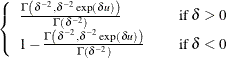
For the generalized gamma distribution, ![]() is computed numerically.
is computed numerically.
The standard errors of the quantile estimates are computed using the estimated covariance matrix of the parameter estimates and a Taylor series expansion of the quantile estimate. The standard error is computed as
|
|
where ![]() is the estimated covariance matrix of the parameter vector
is the estimated covariance matrix of the parameter vector ![]() , and
, and ![]() is the vector
is the vector
![\[ \mb {z} = \left[ \begin{array}{c} \mb {x} \\[0.05in] \hat{u}_ p \\[0.05in] \hat{\sigma } \frac{\partial u_ p}{\partial \delta } \\ \end{array} \right] \]](images/statug_lifereg0198.png) |
where ![]() is the vector of the shape parameters. Unless the NOLOG option is specified, this standard error estimate is converted into
a standard error estimate for
is the vector of the shape parameters. Unless the NOLOG option is specified, this standard error estimate is converted into
a standard error estimate for ![]() as
as ![]() STD. It might be more desirable to compute confidence limits for the log response and convert them back to the original response
variable than to use the standard error estimates for
STD. It might be more desirable to compute confidence limits for the log response and convert them back to the original response
variable than to use the standard error estimates for ![]() directly. See Example 51.1 for a 90% confidence interval of the response constructed by exponentiating a confidence interval for the log response.
directly. See Example 51.1 for a 90% confidence interval of the response constructed by exponentiating a confidence interval for the log response.
The variable CDF is computed as
|
|
where the residual is defined by
|
|
and F is the baseline cumulative distribution function. If the data are interval-censored, then the cumulative distribution function,
![]() , is evaluated at the lower interval endpoint.
, is evaluated at the lower interval endpoint.