Introductory Example: Linear Regression
Regression analysis is the analysis of the relationship between a response or outcome variable and another set of variables. The relationship is expressed through a statistical model equation that predicts a response variable (also called a dependent variable or criterion) from a function of regressor variables (also called independent variables, predictors, explanatory variables, factors, or carriers) and parameters. In a linear regression model the predictor function is linear in the parameters (but not necessarily linear in the regressor variables). The parameters are estimated so that a measure of fit is optimized. For example, the equation for the ith observation might be
|
|
where ![]() is the response variable,
is the response variable, ![]() is a regressor variable,
is a regressor variable, ![]() and
and ![]() are unknown parameters to be estimated, and
are unknown parameters to be estimated, and ![]() is an error term. This model is termed the simple linear regression (SLR) model, because it is linear in
is an error term. This model is termed the simple linear regression (SLR) model, because it is linear in ![]() and
and ![]() and contains only a single regressor variable.
and contains only a single regressor variable.
Suppose you are using regression analysis to relate a child’s weight to a child’s height. One application of a regression
model with the response variable Weight is to predict a child’s weight for a known height. Suppose you collect data by measuring heights and weights of 19 randomly
selected schoolchildren. A simple linear regression model with the response variable weight and the regressor variable height
can be written as
|
|
where

-
is the response variable for the ith child

-
is the regressor variable for the ith child
 ,
, 
-
are the unknown regression parameters

-
is the unobservable random error associated with the ith observation
The data set sashelp.class, which is available in the Sashelp library, identifies the children and their observed heights (variable Height) and weights (variable Weight). The following statements perform the regression analysis:
ods graphics on;
proc reg data=sashelp.class;
   model Weight = Height;
run;
Figure 4.1 displays the default tabular output of the REG procedure for this model. Nineteen observations are read from the data set
and all observations are used in the analysis. The estimates of the two regression parameters are ![]() and
and ![]() . These estimates are obtained by the least squares principle. See the sections Classical Estimation Principles and Linear Model Theory in Chapter 3: Introduction to Statistical Modeling with SAS/STAT Software, for details about the principle of least squares estimation and its role in linear model analysis. For a general discussion
of the theory of least squares estimation of linear models and its application to regression and analysis of variance, refer
to one of the applied regression texts, including Draper and Smith (1981); Daniel and Wood (1980); Johnston (1972); Weisberg (1985).
. These estimates are obtained by the least squares principle. See the sections Classical Estimation Principles and Linear Model Theory in Chapter 3: Introduction to Statistical Modeling with SAS/STAT Software, for details about the principle of least squares estimation and its role in linear model analysis. For a general discussion
of the theory of least squares estimation of linear models and its application to regression and analysis of variance, refer
to one of the applied regression texts, including Draper and Smith (1981); Daniel and Wood (1980); Johnston (1972); Weisberg (1985).
Figure 4.1: Regression for Weight and Height Data
| Number of Observations Read | 19 |
|---|---|
| Number of Observations Used | 19 |
| Analysis of Variance | |||||
|---|---|---|---|---|---|
| Source | DF | Sum of Squares |
Mean Square |
F Value | Pr > F |
| Model | 1 | 7193.24912 | 7193.24912 | 57.08 | <.0001 |
| Error | 17 | 2142.48772 | 126.02869 | ||
| Corrected Total | 18 | 9335.73684 | |||
| Root MSE | 11.22625 | R-Square | 0.7705 |
|---|---|---|---|
| Dependent Mean | 100.02632 | Adj R-Sq | 0.7570 |
| Coeff Var | 11.22330 |
| Parameter Estimates | |||||
|---|---|---|---|---|---|
| Variable | DF | Parameter Estimate |
Standard Error |
t Value | Pr > |t| |
| Intercept | 1 | -143.02692 | 32.27459 | -4.43 | 0.0004 |
| Height | 1 | 3.89903 | 0.51609 | 7.55 | <.0001 |
Based on the least squares estimates shown in Figure 4.1, the fitted regression line relating height to weight is described by the equation
|
|
The “hat” notation is used to emphasize that ![]() is not one of the original observations but a value predicted under the regression model that has been fit to the data. At
the least squares solution the residual sum of squares
is not one of the original observations but a value predicted under the regression model that has been fit to the data. At
the least squares solution the residual sum of squares
|
|
is minimized and the achieved criterion value is displayed in the analysis of variance table as the error sum of squares (2142.48772).
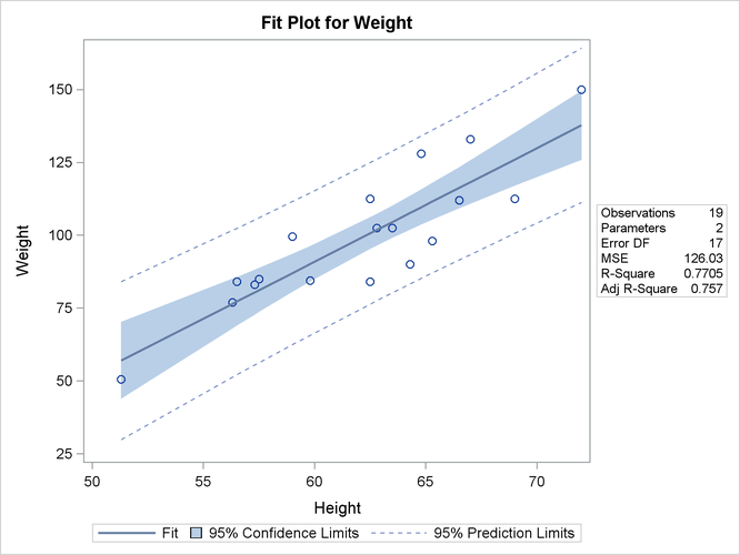
Figure 4.2 displays the fit plot produced by ODS Graphics. The fit plot shows the positive slope of the fitted line. The average weight
of a child changes by ![]() units for each unit change in height. The 95% confidence limits in the fit plot are pointwise limits that cover the mean
weight for a particular height with probability 0.95. The prediction limits, which are wider than the confidence limits, show
the pointwise limits that cover a new observation for a given height with probability 0.95.
units for each unit change in height. The 95% confidence limits in the fit plot are pointwise limits that cover the mean
weight for a particular height with probability 0.95. The prediction limits, which are wider than the confidence limits, show
the pointwise limits that cover a new observation for a given height with probability 0.95.
Figure 4.2: Fit Plot for Regression of Weight on Height
Regression is often used in an exploratory fashion to look for empirical relationships, such as the relationship between Height and Weight. In this example, Height is not the cause of Weight. You would need a controlled experiment to confirm the relationship scientifically. See the section Comments on Interpreting Regression Statistics for more information. A separate question from a possible cause-and-effect relationship between the two variables involved
in this regression is whether the simple linear regression model adequately describes the relationship in these data. If the
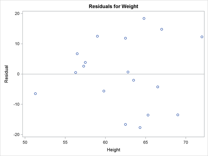
usual assumptions about the model errors ![]() are met in the SLR model, then the errors should have zero mean and equal variance and be uncorrelated. Because the children
were randomly selected, the observations from different children are not correlated. If the mean function of the model is
correctly specified, the fitted residuals
are met in the SLR model, then the errors should have zero mean and equal variance and be uncorrelated. Because the children
were randomly selected, the observations from different children are not correlated. If the mean function of the model is
correctly specified, the fitted residuals ![]() should scatter about the zero reference line without discernible structure. The residual plot in Figure 4.3 confirms this behavior.
should scatter about the zero reference line without discernible structure. The residual plot in Figure 4.3 confirms this behavior.
Figure 4.3: Residual Plot for Regression of Weight on Height
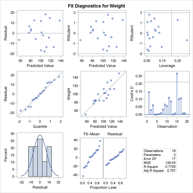
An even more detailed look at the model-data agreement is gained with the panel of regression diagnostics in Figure 4.4. The graph in the upper left panel repeats the raw residual plot in Figure 4.3. The plot of the RSTUDENT residuals shows externally studentized residuals that take into account heterogeneity in the variability of the residuals. RSTUDENT residuals
that exceed the threshold values of ![]() often indicate outlying observations. The residual-by-leverage plot shows that two observations have high leverage—that is, they are unusual in their height values relative to the other children. The normal-probability Q-Q plot
in the second row of the panel shows that the normality assumption for the residuals is reasonable. The plot of the Cook’s D statistic shows that observation 15 exceeds the threshold value; this indicates that the observation for this child is influential
on the regression parameter estimates.
often indicate outlying observations. The residual-by-leverage plot shows that two observations have high leverage—that is, they are unusual in their height values relative to the other children. The normal-probability Q-Q plot
in the second row of the panel shows that the normality assumption for the residuals is reasonable. The plot of the Cook’s D statistic shows that observation 15 exceeds the threshold value; this indicates that the observation for this child is influential
on the regression parameter estimates.
Figure 4.4: Panel of Regression Diagnostics
For detailed information about the interpretation of regression diagnostics and about ODS statistical graphics with the REG procedure, see Chapter 79: The REG Procedure.
SAS/STAT regression procedures produce the following information for a typical regression analysis:
-
parameter estimates derived by using the least squares criterion
-
estimates of the variance of the error term
-
estimates of the variance or standard deviation of the sampling distribution of the parameter estimates
-
tests of hypotheses about the parameters
SAS/STAT regression procedures can produce many other specialized diagnostic statistics, including the following:
-
collinearity diagnostics to measure how strongly regressors are related to other regressors and how this affects the stability and variance of the estimates (REG)
-
influence diagnostics to measure how each individual observation contributes to determining the parameter estimates, the SSE, and the fitted values (LOGISTIC, MIXED, REG, RSREG)
-
lack-of-fit diagnostics that measure the lack of fit of the regression model by comparing the error variance estimate to another pure error variance that is not dependent on the form of the model (CATMOD, PROBIT, RSREG)
-
diagnostic scatter plots that check the fit of the model and highlighted scatter plots that identify particular observations or groups of observations (REG)
-
predicted and residual values, and confidence intervals for the mean and for an individual value (GLM, LOGISTIC, REG)
-
time series diagnostics for equally spaced time series data that measure how much errors might be related across neighboring observations. These diagnostics can also measure functional goodness of fit for data that are sorted by regressor or response variables (REG, SAS/ETS procedures).
Many SAS/STAT procedures produce general and specialized statistical graphics through ODS Graphics to diagnose the fit of the model and the model-data agreement, and to highlight observations that are influential on the analysis. Figure 4.2 and Figure 4.3, for example, are two of the ODS statistical graphs produced by the REG procedure by default for the simple linear regression model. For general information about ODS Graphics, see Chapter 21: Statistical Graphics Using ODS. For specific information about the ODS statistical graphs available with a SAS/STAT procedure, see the PLOTS option in the “Syntax” section for the PROC statement and the “ODS Table Names” section in the “Details” section of the individual procedure documentation.