The VARIOGRAM Procedure

Example 98.2 An Anisotropic Case Study with Surface Trend in the Data
This example shows how to examine data for nonrandom surface trends and anisotropy. You use simulated data where the variable is atmospheric ozone (O ) concentrations measured in Dobson units (DU). The coordinates are offsets from a point in the southwest corner of the measurement area, with the east and north distances in units of kilometers (km). You work with the ozoneSet data set that contains 300 measurements in a square area of 100 km
  100 km.
The following statements read the data set:
title 'Semivariogram Analysis in Anisotropic Case With Trend Removal';

data ozoneSet;
   input East North Ozone @@;
   datalines;
   34.9 68.2 286  39.2 12.5 270  44.4 37.7 275  90.5 27.0 282
   91.1 40.8 285  98.6 61.6 294  61.8 26.7 281  64.0 11.5 274
   22.4 26.5 274  89.3 18.3 279  32.3 28.3 274  31.1 53.1 279
   43.0 17.5 272  79.3 42.3 283  99.9 57.9 291   1.8 24.1 273
   81.7 73.5 294  22.9 32.0 273  64.9 67.5 292  76.5 56.3 285
   78.7 11.7 276  61.8 99.3 307  49.1 86.6 299  40.0 35.8 273
   69.3  3.8 278  23.4  9.3 270  66.3 94.3 304  71.3  6.5 275
    9.7 54.4 280  85.2 81.7 300  30.3 60.9 284  94.6 94.3 309
   10.6 10.3 271  73.0 43.0 280   4.9 50.7 280  19.0 79.4 289
    2.4 73.1 287  77.7 25.2 278   8.4 27.1 276  93.5 19.7 279
    0.2 34.5 275  50.4 91.3 302  55.7 26.2 279  50.3  2.3 274
   16.3 84.4 293  19.0  6.9 272  57.1 92.3 303  61.0  0.4 275
   10.7 18.7 271  15.2 43.5 277  67.0 87.4 301  79.0 54.0 285
   36.0 53.3 279  58.3 52.1 282  56.6 79.7 294  40.4 32.4 275
   48.9 64.1 286  54.0 54.9 281  27.5 48.5 279  36.4 30.3 275
   10.5 31.0 273  87.0 39.4 283  47.9 37.5 274  64.7 63.4 288
    0.5 90.8 294  22.8 22.4 275  31.1 78.8 291  93.6 49.8 290
    2.5 39.3 273  83.6 25.6 282  49.8 24.1 278  73.1 91.8 305
   30.5 90.6 297  26.0 61.2 284  58.4 66.2 289  30.5  4.3 273
   38.3 85.6 298  89.2 96.6 309  53.4  6.3 275  27.3 12.8 271
   43.4 56.5 281  99.5 86.9 305  85.8 22.8 281  83.0 10.9 278
   24.8 16.7 271  51.1 18.8 275  59.0 54.3 283  35.5 91.4 298
   18.1 56.0 279  78.0 36.4 277  56.8  6.9 275  21.1 44.5 277
   73.9 75.9 296  54.2  0.1 274  33.2 75.1 290  38.2  3.3 274
   15.2 14.7 272  15.9 84.2 292  60.2 95.2 304   9.8 27.2 276
   91.2 56.4 289  94.7 86.9 303  56.7 49.6 281  24.2  9.5 270
   43.0 17.0 272  85.9 10.7 278  53.9 41.1 276  30.4 63.4 286
   62.8 86.3 299  76.8 24.6 279  31.6 94.0 300  26.9 73.8 287
   18.9 68.4 284  99.4 37.2 285  79.1  3.3 277  34.9 74.7 289
    6.4 33.8 277  48.4 82.2 294  86.0 58.0 289  92.0 60.4 293
   50.2 91.6 300  12.2 38.3 275  72.7 48.9 283  82.7 34.1 279
   77.0 51.0 286  86.6 15.8 278  42.0 42.7 277  99.3  8.2 278
   17.4 70.6 286  11.2 92.4 295  60.2 28.8 280  92.0 73.3 297
   25.3 30.6 273  36.6  8.9 274  34.2  4.4 273  26.6 54.7 278
    1.7 27.4 278  49.6  1.1 275  62.8 89.3 301  28.0 49.3 279
   51.2 75.1 293  59.3 93.5 304  83.6 90.5 304  79.4 87.0 302
   78.0 28.3 281  16.8 19.1 272   9.1 81.2 292  23.7 55.8 277
   75.5 21.3 279  64.4 43.3 279  38.9 98.9 303  22.5 87.9 293
   96.7 37.9 285  92.3 93.9 308  16.9 25.4 273  15.2 61.5 283
   73.8 94.0 306  57.4 97.2 305  73.2  4.9 276  39.2 82.3 294
   95.7 99.4 315  66.0 98.4 306  95.3 26.9 283  45.4 75.3 291
   64.8 15.4 276  69.8 55.4 284  36.3 74.9 290   9.9 22.2 276
   65.8 13.9 276  13.0 82.0 293  95.6 77.2 301  32.5 55.6 279
   45.8 35.5 275  62.2  6.6 274  25.2 51.2 279  92.4  8.1 277
   40.5 35.3 273   9.9  3.9 271  43.5 44.0 278  68.6 61.3 287
   64.2 77.5 296  57.6 81.6 294  69.5 64.7 291  64.3 95.1 304
    2.8 62.4 283  33.2 83.3 294  10.7 71.0 285  24.3 88.2 294
   94.5 32.2 283  21.0 67.6 286  20.1 71.6 286  85.2 71.3 296
   94.8 30.7 283  53.4 92.0 301  81.0 50.0 287  54.6 29.9 277
   71.1 90.1 303  15.2  2.9 271  83.6 17.8 278  76.0 21.8 279
   55.6 37.4 275  86.7 83.7 303  43.6 83.6 295  44.2 31.7 274
   90.0 83.3 300   6.2  0.5 270  42.2 87.7 298  31.7  4.3 273
   91.4 41.2 285  78.0 50.6 286  27.1 56.1 278  72.6 63.9 291
   29.3 49.9 281  49.0 36.9 275  13.9 53.5 280  93.1 83.2 300
   73.0 61.6 289  63.1 27.5 280  38.3 72.5 287  72.7 34.2 277
    6.9 32.3 274  17.1 58.6 280  19.6 94.6 297   2.7 36.5 276
   34.5  5.5 275  98.6 95.9 313   9.1 71.1 285  88.6 55.8 287
   26.8 78.5 289  64.8 66.6 292  59.7 25.7 280  47.3 70.2 288
    6.1 94.4 296  50.5 82.7 296   9.1 41.6 276  86.0 71.0 296
   75.2 69.8 293  73.3 84.8 300  42.5 15.9 274  56.1 76.1 292
   87.9 41.2 285  65.1  9.8 274  79.0 41.2 282  44.6 65.1 287
   54.7 68.3 289  57.0 26.8 279   8.7 12.3 270  33.7 61.9 286
   25.0 55.8 278  69.3 94.9 306  49.2 64.6 287  78.2 93.7 307
   47.9 26.6 277  96.9 51.4 292  39.6 73.4 287  37.9 66.1 285
   94.5 71.4 296  51.6 18.3 276  37.6 73.2 287  68.5 10.7 274
   46.7  9.6 273  87.4 38.9 282  45.6 43.9 277  70.7 76.9 296
   82.8 53.6 287  82.5 55.4 286  37.8  5.1 275  89.8 96.1 309
   63.9  4.9 276   2.0 11.7 270  31.3 59.2 282  93.9 65.3 296
   47.9 93.0 301  29.9 36.0 274  14.6 28.3 274  17.5 70.1 286
    2.6 68.5 282  23.1 12.0 268  36.8 20.4 273  80.9  9.0 276
   39.2  0.0 274  26.2 44.3 276  81.9 12.9 277   3.2 21.4 272
   76.9 76.7 297  88.6  7.7 277   9.7  8.4 273  26.7 91.5 296
   73.8  6.1 276  33.7 39.3 276  64.0 58.4 286   5.7 91.2 295
   85.8 93.8 307  85.8 39.1 281  93.9 63.4 295  53.1 46.3 278
   51.9 42.9 277  16.8 75.7 288  29.2 66.9 285  37.4 72.5 287
   ;
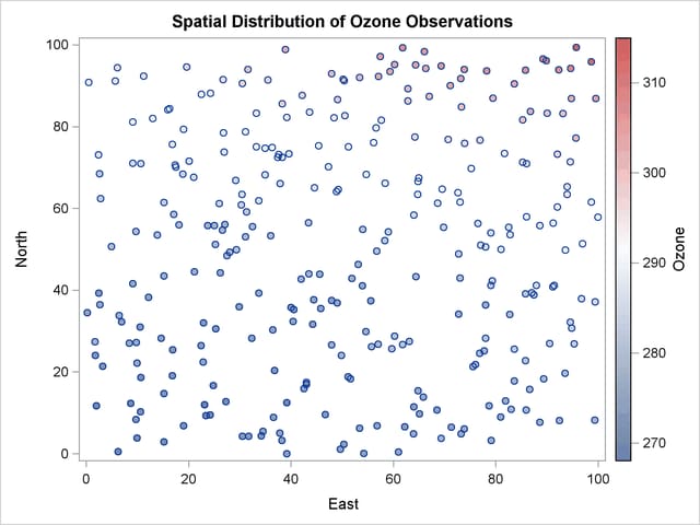
The initial step is to explore the data set by inspecting the data spatial distribution. Run PROC VARIOGRAM, specifying the NOVARIOGRAM option in the COMPUTE statement as follows:
ods graphics on;
proc variogram data=ozoneSet;
   compute novariogram nhc=35;
   coord xc=East yc=North;
   var Ozone;
run;
The result is a scatter plot of the observed data shown in Output 98.2.1. The scatter plot suggests an almost uniform spread of the measurements throughout the prediction area. No direct inference can be made about the existence of a surface trend in the data. However, the apparent stratification of ozone values in the northeast–southwest direction might indicate a nonrandom trend.
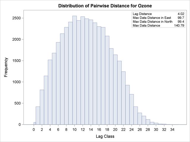
You need to define the size and count of the data classes by specifying suitable values for the LAGDISTANCE= and MAXLAGS= options, respectively. Compared to the smaller sample of thickness data used in Getting Started: VARIOGRAM Procedure, the larger size of the ozoneSet data results in more densely populated distance classes for the same value of the NHCLASSES= option. After you experiment with a variety of values for the NHCLASSES= option, you can adjust LAGDISTANCE= to have a relatively small number. Then you can account for a large value of MAXLAGS= so that you obtain many sample semivariogram points within your data correlation range. Specifying these values requires some exploration, for which you might need to return to this point from a later stage in your semivariogram analysis. For illustration purposes you now specify NHCLASSES=35.
Your choice of NHCLASSES=35 yields the pairwise distance intervals table in Output 98.2.2 and the corresponding histogram in Output 98.2.3.
| Pairwise Distance Intervals | ||||
|---|---|---|---|---|
| Lag Class |
Bounds | Number of Pairs | Percentage of Pairs |
|
| 0 | 0.00 | 2.01 | 52 | 0.12% |
| 1 | 2.01 | 6.03 | 420 | 0.94% |
| 2 | 6.03 | 10.06 | 815 | 1.82% |
| 3 | 10.06 | 14.08 | 1143 | 2.55% |
| 4 | 14.08 | 18.10 | 1518 | 3.38% |
| 5 | 18.10 | 22.12 | 1680 | 3.75% |
| 6 | 22.12 | 26.15 | 1931 | 4.31% |
| 7 | 26.15 | 30.17 | 2135 | 4.76% |
| 8 | 30.17 | 34.19 | 2285 | 5.09% |
| 9 | 34.19 | 38.21 | 2408 | 5.37% |
| 10 | 38.21 | 42.24 | 2551 | 5.69% |
| 11 | 42.24 | 46.26 | 2444 | 5.45% |
| 12 | 46.26 | 50.28 | 2535 | 5.65% |
| 13 | 50.28 | 54.30 | 2487 | 5.55% |
| 14 | 54.30 | 58.33 | 2460 | 5.48% |
| 15 | 58.33 | 62.35 | 2391 | 5.33% |
| 16 | 62.35 | 66.37 | 2302 | 5.13% |
| 17 | 66.37 | 70.39 | 2285 | 5.09% |
| 18 | 70.39 | 74.41 | 2079 | 4.64% |
| 19 | 74.41 | 78.44 | 1786 | 3.98% |
| 20 | 78.44 | 82.46 | 1640 | 3.66% |
| 21 | 82.46 | 86.48 | 1493 | 3.33% |
| 22 | 86.48 | 90.50 | 1243 | 2.77% |
| 23 | 90.50 | 94.53 | 925 | 2.06% |
| 24 | 94.53 | 98.55 | 710 | 1.58% |
| 25 | 98.55 | 102.57 | 421 | 0.94% |
| 26 | 102.57 | 106.59 | 274 | 0.61% |
| 27 | 106.59 | 110.62 | 200 | 0.45% |
| 28 | 110.62 | 114.64 | 120 | 0.27% |
| 29 | 114.64 | 118.66 | 55 | 0.12% |
| 30 | 118.66 | 122.68 | 35 | 0.08% |
| 31 | 122.68 | 126.71 | 14 | 0.03% |
| 32 | 126.71 | 130.73 | 11 | 0.02% |
| 33 | 130.73 | 134.75 | 2 | 0.00% |
| 34 | 134.75 | 138.77 | 0 | 0.00% |
| 35 | 138.77 | 142.80 | 0 | 0.00% |
Notice the overall high pair count in the majority of classes in Output 98.2.2. You can see that even for higher values of NHCLASSES= the classes are still sufficiently populated for your semivariogram analysis according to the rule of thumb stated in the section Choosing the Size of Classes. Based on the displayed information in Output 98.2.3, you specify LAGDISTANCE=4 km. You can further experiment with smaller lag sizes to obtain more points in your sample semivariogram.
You can focus on the MAXLAGS= specification at a later point. The important step now is to investigate the presence of trends in the measurement. The following section makes a suggestion about how to remove surface trends from your data and then continues the semivariogram analysis with the detrended data.