The VARIOGRAM Procedure

| Empirical Semivariogram Computation |
Using the values of LAGDISTANCE=7 and MAXLAGS=10 computed previously, rerun PROC VARIOGRAM without the NOVARIOGRAM option in order to compute the empirical semivariogram. You specify the CL option in the COMPUTE statement to calculate the 95% confidence limits for the classical semivariance. The section COMPUTE Statement describes how to use the ALPHA= option to specify a different confidence level.
Also, you can request a robust version of the semivariance with the ROBUST option in the COMPUTE statement. PROC VARIOGRAM produces a plot that shows both the classical and the robust empirical semivariograms. See the details of the PLOTS option to specify different instances of plots of the empirical semivariogram. The following statements implement the preceding requests:
proc variogram data=thick outv=outv;
   compute lagd=7 maxlag=10 cl robust;
   coordinates xc=East yc=North;
   var Thick;
run;
Figure 98.6 displays the PROC VARIOGRAM output empirical semivariogram table for the preceding statements. The table displays a total of eleven lag classes, even though you specified MAXLAGS=10. The VARIOGRAM procedure always includes a zero lag class in the computations in addition to the MAXLAGS classes you request with the MAXLAGS= option. Hence, semivariance is actually computed at MAXLAGS 1 lag classes; see the section Distance Classification for more details.
| Spatial Correlation Analysis with PROC VARIOGRAM |
| Empirical Semivariogram | |||||||
|---|---|---|---|---|---|---|---|
| Lag Class |
Pair Count |
Average Distance |
Semivariance | ||||
| Robust | Classical | Standard Error |
95% Confidence Limits | ||||
| 0 | 7 | 2.64 | 0.028 | 0.034 | 0.018 | 0 | 0.069 |
| 1 | 82 | 7.29 | 0.210 | 0.394 | 0.061 | 0.273 | 0.514 |
| 2 | 138 | 14.16 | 1.008 | 1.179 | 0.142 | 0.901 | 1.458 |
| 3 | 169 | 21.08 | 3.018 | 2.799 | 0.304 | 2.202 | 3.396 |
| 4 | 205 | 27.93 | 4.811 | 4.602 | 0.455 | 3.711 | 5.493 |
| 5 | 213 | 35.17 | 5.990 | 5.928 | 0.574 | 4.802 | 7.054 |
| 6 | 214 | 42.20 | 8.104 | 7.518 | 0.727 | 6.094 | 8.943 |
| 7 | 250 | 48.78 | 7.533 | 7.221 | 0.646 | 5.955 | 8.487 |
| 8 | 247 | 56.16 | 8.066 | 7.195 | 0.647 | 5.926 | 8.464 |
| 9 | 281 | 62.89 | 8.279 | 6.845 | 0.577 | 5.713 | 7.976 |
| 10 | 250 | 69.93 | 8.144 | 6.358 | 0.569 | 5.243 | 7.472 |
Figure 98.7 shows both the classical and robust empirical semivariograms. In addition, the plot features the approximate 95% confidence limits for the classical semivariance. The figure exhibits a typical behavior of the computed semivariance uncertainty, where in general the variance increases with distance from the origin at Distance=0.
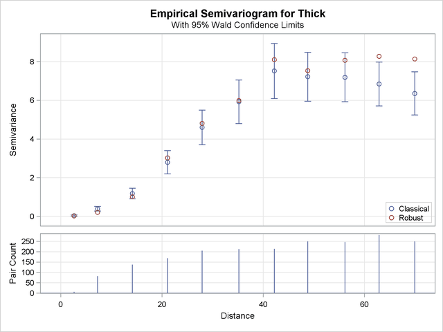
The needle plot in the lower part of the Figure 98.7 provides the number of pairs that were used in the computation of the empirical semivariance for each lag class shown. In general, this is a pairwise distribution that is different from the distribution depicted in Figure 98.4. First, the number of pairs shown in the needle plot depends on the particular criteria you specify in the COMPUTE statement of PROC VARIOGRAM. Second, the distances shown for each lag on the Distance axis are not the midpoints of the lag classes as in the pairwise distances plot, but rather the average distance from the origin Distance=0 of all pairs in a given lag class.