The NLIN Procedure
- Overview
-
Getting Started

-
Syntax
-
Details
Automatic Derivatives Measures of Nonlinearity and Diagnostics Missing Values Special Variables Troubleshooting Computational Methods Output Data Sets Confidence Intervals Covariance Matrix of Parameter Estimates Convergence Measures Displayed Output Incompatibilities with SAS 6.11 and Earlier Versions of PROC NLIN ODS Table Names ODS Graphics
-
Examples
- References
Example 62.5 Comparing Nonlinear Trends among Groups
When you model nonlinear trends in the presence of group (classification) variables, two questions often arise: whether the trends should be varied by group, and how to decide which parameters should be varied across groups. A large battery of tools is available on linear statistical models to test hypotheses involving the model parameters, especially to test linear hypotheses. To test similar hypotheses in nonlinear models, you can draw on analogous tools. Especially important in this regard are comparisons of nested models by contrasting their residual sums of squares.
In this example, a two-group model from a pharmacokinetic application is fit to data that are in part based on the theophylline data from Pinheiro and Bates (1995) and the first example in the documentation for the NLMIXED procedure. In a pharmacokinetic application you study how a drug is dispersed through a living organism. The following data represent concentrations of the drug theophylline over a 25-hour period following oral administration. The data are derived by collapsing and averaging the subject-specific data from Pinheiro and Bates (1995) in a particular, yet unimportant, way. The purpose of arranging the data in this way is purely to demonstrate the methodology.
data theop;
  input time dose conc @@;
  if (dose = 4) then group=1; else group=2;
  datalines;
 0.00   4  0.1633  0.25   4   2.045
 0.27   4     4.4  0.30   4    7.37
 0.35   4    1.89  0.37   4    2.89
 0.50   4    3.96  0.57   4    6.57
 0.58   4     6.9  0.60   4     4.6
 0.63   4    9.03  0.77   4    5.22
 1.00   4    7.82  1.02   4   7.305
 1.05   4    7.14  1.07   4     8.6
 1.12   4    10.5  2.00   4    9.72
 2.02   4    7.93  2.05   4    7.83
 2.13   4    8.38  3.50   4    7.54
 3.52   4    9.75  3.53   4    5.66
 3.55   4   10.21  3.62   4     7.5
 3.82   4    8.58  5.02   4   6.275
 5.05   4    9.18  5.07   4    8.57
 5.08   4     6.2  5.10   4    8.36
 7.02   4    5.78  7.03   4    7.47
 7.07   4   5.945  7.08   4    8.02
 7.17   4    4.24  8.80   4    4.11
 9.00   4     4.9  9.02   4    5.33
 9.03   4    6.11  9.05   4    6.89
 9.38   4    7.14 11.60   4    3.16
11.98   4    4.19 12.05   4    4.57
12.10   4    5.68 12.12   4    5.94
12.15   4     3.7 23.70   4    2.42
24.15   4    1.17 24.17   4    1.05
24.37   4    3.28 24.43   4    1.12
24.65   4    1.15  0.00   5   0.025
 0.25   5    2.92  0.27   5   1.505
 0.30   5    2.02  0.50   5   4.795
 0.52   5    5.53  0.58   5    3.08
 0.98   5   7.655  1.00   5   9.855
 1.02   5    5.02  1.15   5    6.44
 1.92   5    8.33  1.98   5    6.81
 2.02   5  7.8233  2.03   5    6.32
 3.48   5    7.09  3.50   5   7.795
 3.53   5    6.59  3.57   5    5.53
 3.60   5    5.87  5.00   5     5.8
 5.02   5  6.2867  5.05   5    5.88
 6.98   5    5.25  7.00   5    4.02
 7.02   5    7.09  7.03   5   4.925
 7.15   5    4.73  9.00   5    4.47
 9.03   5    3.62  9.07   5    4.57
 9.10   5     5.9  9.22   5    3.46
12.00   5    3.69 12.05   5    3.53
12.10   5    2.89 12.12   5    2.69
23.85   5    0.92 24.08   5    0.86
24.12   5    1.25 24.22   5    1.15
24.30   5     0.9 24.35   5    1.57
;
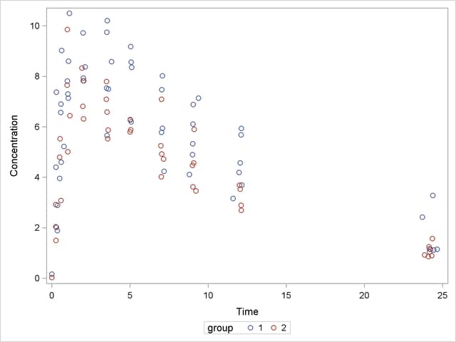
The following code plots the theophylline concentration data over time for the two groups (Output 62.5.1). In each group the concentration tends to rise sharply right after the drug is administered, followed by a prolonged tapering of the concentration.
proc sgplot data=theop;
   scatter x=time y=conc / group=group;
   yaxis label='Concentration';
   xaxis label='Time';
run;
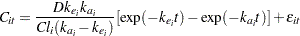
In the context of nonlinear mixed models, Pinheiro and Bates (1995) consider a first-order compartment model for these data. In terms of two fixed treatment groups, the model can be written as
 |
where  is the observed concentration in group
  at time
  ,
,  is the dose of theophylline,
  is the elimination rate in group ,
  is the absorption rate in group ,
  is the clearance in group , and
  denotes the model error. Because the rates and the clearance must be positive, you can parameterize the model in terms of log rates and the log clearance:
 |
 |
|||
 |
 |
|||
 |
 |
In this parameterization the model contains six parameters, and the rates and clearance vary by group. This produces two separate response profiles, one for each group. On the other extreme, you could model the trends as if there were no differences among the groups:
|
 |
|||
|
 |
|||
|
 |
In between these two extremes lie other models, such as a model where both groups have the same absorption and elimination rate, but different clearances. The question then becomes how to go about building a model in an organized manner.
To test hypotheses about nested nonlinear models, you can apply the idea of a "Sum of Squares Reduction Test." A reduced model is nested within a full model if you can impose  constraints on the full model to obtain the reduced model. Then, if
  and
and  denote the residual sum of squares in the reduced and the full model, respectively, the test statistic is
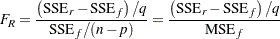 |
where  are the number of observations used and
  are the number of parameters in the full model. The numerator of the
  statistic is the average reduction in residual sum of squares per constraint. The mean squared error of the full model is used to scale this average because it is less likely to be a biased estimator of the residual variance than the variance estimate from a constrained (reduced) model. The statistic is then compared against quantiles from an
  distribution with numerator and
  denominator degrees of freedom. Schabenberger and Pierce (2002) discuss the justification for this test and compare it to other tests in nonlinear models.
In the present application we might phrase the initial question akin to the overall F test for a factor in a linear model: Should any parameters be varied between the two groups? The corresponding null hypothesis is
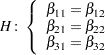 |
where the first subscript identifies the type of the parameter and the second subscript identifies the group. Note that this hypothesis implies
 |
If you fail to reject this hypothesis, there is no need to further examine individual parameter differences.
The reduced model—the model subject to the null hypothesis—is fit with the following PROC NLIN statements:
proc nlin data=theop;
   parms beta1=-3.22 beta2=0.47 beta3=-2.45;
   cl   = exp(beta1);
   ka   = exp(beta2);
   ke   = exp(beta3);
   mean = dose*ke*ka*(exp(-ke*time)-exp(-ka*time))/cl/(ka-ke);
   model conc = mean;
   ods output Anova=aovred(rename=(ss=ssred ms=msred df=dfred));
run;
The clearance, the rates, and the mean function are formed independently of the group membership. The analysis of variance table is saved to the data set aovred, and some of its variables are renamed. This is done so that the data set can be merged easily with the analysis of variance table for the full model (see following).
The converged model has a residual sum of square of  and a mean squared error of
  (Output 62.5.2). The table of parameter estimates gives the values for the estimated log clearance
  , the estimated log absorption rate
  , and the estimated log elimination rate
  .
.
| NOTE: Convergence criterion met. |
| Note: | An intercept was not specified for this model. |
| Source | DF | Sum of Squares | Mean Square | F Value | Approx Pr > F |
|---|---|---|---|---|---|
| Model | 3 | 3100.5 | 1033.5 | 342.87 | <.0001 |
| Error | 95 | 286.4 | 3.0142 | ||
| Uncorrected Total | 98 | 3386.8 |
| Parameter | Estimate | Approx Std Error |
Approximate 95% Confidence Limits |
|
|---|---|---|---|---|
| beta1 | -3.2991 | 0.0956 | -3.4888 | -3.1094 |
| beta2 | 0.4769 | 0.1640 | 0.1512 | 0.8025 |
| beta3 | -2.5555 | 0.1410 | -2.8354 | -2.2755 |
The full model, in which all three parameters are varied by group, can be fit with the following statements in the NLIN procedure:
proc nlin data=theop;
   parms beta1_1=-3.22 beta2_1=0.47 beta3_1=-2.45
         beta1_2=-3.22 beta2_2=0.47 beta3_2=-2.45;
   if (group=1) then do;
      cl   = exp(beta1_1);
      ka   = exp(beta2_1);
      ke   = exp(beta3_1);
   end; else do;
      cl   = exp(beta1_2);
      ka   = exp(beta2_2);
      ke   = exp(beta3_2);
   end;
   mean = dose*ke*ka*(exp(-ke*time)-exp(-ka*time))/cl/(ka-ke);
   model conc = mean;
   ods output Anova=aovfull;
run;
Separate parameters for the groups are now specified in the PARMS statement, and the value of the model variables cl, ka, and ke is assigned conditional on the group membership of an observation. Notice that the same expression as in the previous run can be used to model the mean function.
The results from this PROC NLIN run are shown in Output 62.5.3. The residual sum of squares in the full model is only  , compared to in the reduced model (Output 62.5.3).
| NOTE: Convergence criterion met. |
| Note: | An intercept was not specified for this model. |
| Source | DF | Sum of Squares | Mean Square | F Value | Approx Pr > F |
|---|---|---|---|---|---|
| Model | 6 | 3247.9 | 541.3 | 358.56 | <.0001 |
| Error | 92 | 138.9 | 1.5097 | ||
| Uncorrected Total | 98 | 3386.8 |
| Parameter | Estimate | Approx Std Error |
Approximate 95% Confidence Limits |
|
|---|---|---|---|---|
| beta1_1 | -3.5671 | 0.0864 | -3.7387 | -3.3956 |
| beta2_1 | 0.4421 | 0.1349 | 0.1742 | 0.7101 |
| beta3_1 | -2.6230 | 0.1265 | -2.8742 | -2.3718 |
| beta1_2 | -3.0111 | 0.1061 | -3.2219 | -2.8003 |
| beta2_2 | 0.3977 | 0.1987 | 0.00305 | 0.7924 |
| beta3_2 | -2.4442 | 0.1618 | -2.7655 | -2.1229 |
Whether this reduction in sum of squares is sufficient to declare that the full model provides a significantly better fit than the reduced model depends on the number of constraints imposed on the full model and on the variability in the data. In other words, before drawing any conclusions, you have to take into account how many parameters have been dropped from the model and how much variation around the regression trends the data exhibit. The statistic sets these quantities into relation. The following macro merges the analysis of variance tables from the full and reduced model, and computes and its -value:
%macro SSReductionTest;
   data aov; merge aovred aovfull;
     if (Source='Error') then do;
        Fstat  = ((SSred-SS)/(dfred-df))/ms;
        pvalue = 1-Probf(Fstat,dfred-df,df);
        output;
     end;
   run;
   proc print data=aov label noobs;
      label Fstat  = 'F Value'
            pValue = 'Prob > F';
      format pvalue pvalue8.;
      var Fstat pValue;
   run;
%mend;
%SSReductionTest;
| F Value | Prob > F |
|---|---|
| 32.5589 | <.000001 |
There is clear evidence that the model with separate trends fits these data significantly better (Output 62.5.4). To decide whether all parameters should be varied between the groups or only one or two of them, we first refit the model in a slightly different parameterization:
proc nlin data=theop;
   parms beta1_1=-3.22 beta2_1=0.47 beta3_1=-2.45
         beta1_diff=0 beta2_diff=0 beta3_diff=0;
   if (group=1) then do;
      cl   = exp(beta1_1);
      ka   = exp(beta2_1);
      ke   = exp(beta3_1);
   end; else do;
      cl   = exp(beta1_1 + beta1_diff);
      ka   = exp(beta2_1 + beta2_diff);
      ke   = exp(beta3_1 + beta3_diff);
   end;
   mean = dose*ke*ka*(exp(-ke*time)-exp(-ka*time))/cl/(ka-ke);
   model conc = mean;
run;
In the preceding statements, the parameters in the second group were expressed using offsets from parameters in the first group. For example, the parameter beta1_diff measures the change in log clearance between group 2 and group 1.
This simple reparameterization does not affect the model fit. The analysis of variance tables in Output 62.5.5 and Output 62.5.3 are identical. It does, however, affect the interpretation of the estimated quantities. Since the parameter beta1_diff measures the change in the log clearance rates between the groups, you can use the approximate 95% confidence limits in Output 62.5.5 to assess whether that quantity in the pharmacokinetic equation varies between groups. Only the confidence interval for the difference in the log clearances excludes 0. The intervals for beta2_diff and beta3_diff include 0.
| NOTE: Convergence criterion met. |
| Note: | An intercept was not specified for this model. |
| Source | DF | Sum of Squares | Mean Square | F Value | Approx Pr > F |
|---|---|---|---|---|---|
| Model | 6 | 3247.9 | 541.3 | 358.56 | <.0001 |
| Error | 92 | 138.9 | 1.5097 | ||
| Uncorrected Total | 98 | 3386.8 |
| Parameter | Estimate | Approx Std Error |
Approximate 95% Confidence Limits |
|
|---|---|---|---|---|
| beta1_1 | -3.5671 | 0.0864 | -3.7387 | -3.3956 |
| beta2_1 | 0.4421 | 0.1349 | 0.1742 | 0.7101 |
| beta3_1 | -2.6230 | 0.1265 | -2.8742 | -2.3718 |
| beta1_diff | 0.5560 | 0.1368 | 0.2842 | 0.8278 |
| beta2_diff | -0.0444 | 0.2402 | -0.5214 | 0.4326 |
| beta3_diff | 0.1788 | 0.2054 | -0.2291 | 0.5866 |
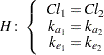
This suggests as the final model one where the absorption and elimination rates are the same for both groups and only the clearances are varied. The following statements fit this model and perform the sum of squares reduction test:
proc nlin data=theop;
   parms beta1_1=-3.22 beta2_1=0.47 beta3_1=-2.45
         beta1_diff=0;
   ka = exp(beta2_1);
   ke = exp(beta3_1);
   if (group=1) then do;
      cl = exp(beta1_1);
   end; else do;
      cl = exp(beta1_1 + beta1_diff);
   end;
   mean = dose*ke*ka*(exp(-ke*time)-exp(-ka*time))/cl/(ka-ke);
   model conc = mean;
   ods output Anova=aovred(rename=(ss=ssred ms=msred df=dfred));
   output out=predvals predicted=p;
run;
%SSReductionTest;
The results for this model with common absorption and elimination rates are shown in Output 62.5.6. The sum-of-squares reduction test comparing this model against the full model with six parameters shows—as expected—that the full model does not fit the data significantly better ( , Output 62.5.7).
| NOTE: Convergence criterion met. |
| Note: | An intercept was not specified for this model. |
| Source | DF | Sum of Squares | Mean Square | F Value | Approx Pr > F |
|---|---|---|---|---|---|
| Model | 4 | 3246.5 | 811.6 | 543.60 | <.0001 |
| Error | 94 | 140.3 | 1.4930 | ||
| Uncorrected Total | 98 | 3386.8 |
| Parameter | Estimate | Approx Std Error |
Approximate 95% Confidence Limits |
|
|---|---|---|---|---|
| beta1_1 | -3.5218 | 0.0681 | -3.6570 | -3.3867 |
| beta2_1 | 0.4226 | 0.1107 | 0.2028 | 0.6424 |
| beta3_1 | -2.5571 | 0.0988 | -2.7532 | -2.3610 |
| beta1_diff | 0.4346 | 0.0454 | 0.3444 | 0.5248 |
| F Value | Prob > F |
|---|---|
| 0.48151 | 0.619398 |
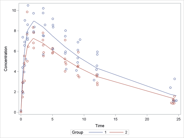
A plot of the observed and predicted values for this final model is obtained with the following statements:
proc sgplot data=predvals;
   scatter x=time y=conc / group=group;
   series  x=time y=p    / group=group name='fit';
   keylegend 'fit'       / across=2 title='Group';
   yaxis label='Concentration';
   xaxis label='Time';
run;
The plot is shown in Output 62.5.8.
The sum-of-squares reduction test is not the only possibility of performing linear-model style hypothesis testing in nonlinear models. You can also perform Wald-type testing of linear hypotheses about the parameter estimates. See Example 40.17 in Chapter 40, The GLIMMIX Procedure, for an application of this example that uses the NLIN and GLIMMIX procedures to compare the parameters across groups and adjusts p-values for multiplicity.