The KDE Procedure

As shown in the last subsection, kernel density estimates can be expressed as a submatrix of a certain convolution. The fast Fourier transform (FFT) is a computationally effective method for computing such convolutions. For a reference on this material, see Press et al. (1988).

The discrete Fourier transform of a complex vector 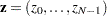is the vector 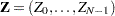, where

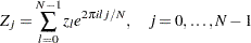and is the square root of . The vector can be recovered from by applying the inverse discrete Fourier transform formula

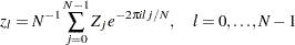Discrete Fourier transforms and their inverses can be computed quickly using the FFT algorithm, especially when is highly composite; that is, it can be decomposed into many factors, such as a power of . By the discrete convolution theorem, the convolution of two vectors is the inverse Fourier transform of the element-by-element product of their Fourier transforms. This, however, requires certain periodicity assumptions, which explains why the vectors and require zero-padding. This is to avoid wrap-around effects (refer to Press et al.; 1988, pp. 410–411). The vector is actually mirror-imaged so that the convolution of and will be the vector of binned estimates. Thus, if denotes the inverse Fourier transform of the element-by-element product of the Fourier transforms of and , then the first elements of are the estimates.

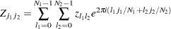
The bivariate Fourier transform of an complex matrix having entry equal to is the matrix with entry given by

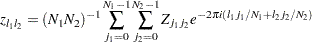
and the formula of the inverse is

The same discrete convolution theorem applies, and zero-padding is needed for matrices and . In the case of , the matrix is mirror-imaged twice. Thus, if denotes the inverse Fourier transform of the element-by-element product of the Fourier transforms of and , then the upper-left corner of contains the estimates.