Some Measurement Models
In the section Regression with Measurement Errors in  and
and  , outcome variables and predictor variables are assumed to have been measured with errors. In order to study the true relationships among the true scores variables, models for measurement errors are also incorporated into the estimation. The context of applications is that of regression or econometric analysis.
In the social and behavioral sciences, the same kind of model is developed in the context of test theory or item construction for measuring cognitive abilities, personality traits, or other latent variables. This kind of modeling is better-known as measurement models or confirmatory factor analysis (these two terms are interchangeable) in the psychometric field. Usually, applications in the social and behavioral sciences involve a much larger number of observed variables. This section considers some of these measurement or confirmatory factor-analytic models. For illustration purposes, only a handful of variables are used in the examples. Applications that use the PATH modeling language in PROC CALIS are described.
H4: Full Measurement Model for Lord Data
Psychometric test theory involves many kinds of models that relate scores on psychological and educational tests to latent variables that represent intelligence or various underlying abilities. The following example uses data on four vocabulary tests from Lord (1957). Tests  and have 15 items each and are administered with very liberal time limits. Tests and
  have 75 items and are administered under time pressure. The covariance matrix is read by the following DATA step:
data lord(type=cov);
   input _type_ $ _name_ $ W X Y Z;
   datalines;
n   . 649       .       .       .
cov W 86.3979   .       .       .
cov X 57.7751 86.2632   .       .
cov Y 56.8651 59.3177 97.2850   .
cov Z 58.8986 59.6683 73.8201 97.8192
;
The psychometric model of interest states that and are determined by a single common factor  , and and are determined by a single common factor
  . The two common factors are expected to have a positive correlation, and it is desired to estimate this correlation. It is convenient to assume that the common factors have unit variance, so their correlation will be equal to their covariance. The error terms for all the manifest variables are assumed to be uncorrelated with each other and with the common factors. The model equations are
 |
 |
 |
|||
 |
|
 |
|||
 |
|
 |
|||
 |
|
 |
with the following assumptions:
 |
|
 |
|||
 |
|
 |
|||
 |
|
 |
|||
 |
|
 |
|||
|
|
 |
|||
|
|
 |
|||
|
|
 |
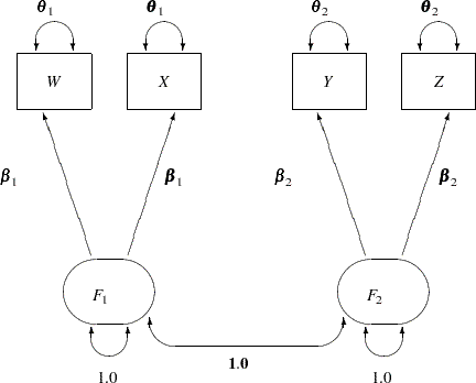
The corresponding path diagram is shown in Figure 17.16.
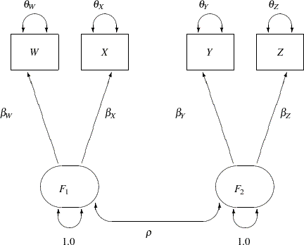
In Figure 17.16, error terms are not explicitly represented, but error variances for the observed variables are represented by double-headed arrows that point to the variables. The error variance parameters in the model are labeled with  ,
,  ,
,  , and
, and  , respectively, for the four observed variables. In the terminology of confirmatory factor analysis, these four variables are called indicators of the corresponding latent factors and .
Figure 17.16 represents the model equations clearly. It includes all the variables and the parameters in the diagram. However, sometimes researchers represent the same model with a simplified path diagram in which unconstrained parameters are not labeled, as shown in Figure 17.17.
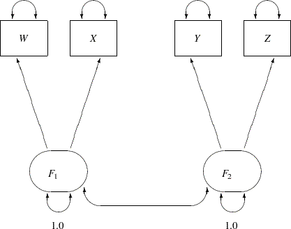
This simplified representation is also compatible with the PATH modeling language of PROC CALIS. In fact, this might be an easier starting point for modelers. With the following rules, the conversion from the path diagram to the PATH model specification is very straightforward:
Each single-headed arrow in the path diagram is specified in the PATH statement.
Each double-headed arrow that points to a single variable is specified in the PVAR statement.
Each double-headed arrow that points to two distinct variables is specified in the PCOV statement.
Hence, you can convert the simplified path diagram in Figure 17.17 easily to the following PATH model specification:
proc calis data=lord;
   path
      W <--- F1,
      X <--- F1,
      Y <--- F2,
      Z <--- F2;
   pvar
      F1 = 1.0,
      F2 = 1.0,
      W X Y Z;
   pcov
      F1 F2;
run;
In this specification, you do not need to specify the parameter names. However, you do need to specify fixed values specified in the path diagram. For example, the variances of F1 and F2 are both fixed at 1 in the PVAR statement.
These fixed variances are applied solely for the purpose of model identification. Because F1 and F2 are latent variables and their scales are arbitrary, fixing their scales are necessary for model identification. Beyond these two identification constraints, none of the parameters in the model is constrained. Therefore, this is referred to as the "full" measurement model for the Lord data.
An annotated fit summary is displayed in Figure 17.18.
| Fit Summary | |
|---|---|
| Chi-Square | 0.7030 |
| Chi-Square DF | 1 |
| Pr > Chi-Square | 0.4018 |
| Standardized RMSR (SRMSR) | 0.0030 |
| Adjusted GFI (AGFI) | 0.9946 |
| RMSEA Estimate | 0.0000 |
| Bentler Comparative Fit Index | 1.0000 |
The chi-square value is 0.7030 ( =1,
=1,  =0.4018). This indicates that you cannot reject the hypothesized model. The standardized root mean square error (SRMSR) is 0.003, which is much smaller than the conventional 0.05 value for accepting good model fit. Similarly, the RMSEA value is virtually zero, indicating an excellent fit. The adjusted GFI (AGFI) and Bentler comparative fit index are close to 1, which also indicate an excellent model fit.
The estimation results are displayed in Figure 17.19.
| PATH List | ||||||
|---|---|---|---|---|---|---|
| Path | Parameter | Estimate | Standard Error |
t Value | ||
| W | <--- | F1 | _Parm1 | 7.50066 | 0.32339 | 23.19390 |
| X | <--- | F1 | _Parm2 | 7.70266 | 0.32063 | 24.02354 |
| Y | <--- | F2 | _Parm3 | 8.50947 | 0.32694 | 26.02730 |
| Z | <--- | F2 | _Parm4 | 8.67505 | 0.32560 | 26.64301 |
| Variance Parameters | |||||
|---|---|---|---|---|---|
| Variance Type |
Variable | Parameter | Estimate | Standard Error |
t Value |
| Exogenous | F1 | 1.00000 | |||
| F2 | 1.00000 | ||||
| Error | W | _Parm5 | 30.13796 | 2.47037 | 12.19979 |
| X | _Parm6 | 26.93217 | 2.43065 | 11.08021 | |
| Y | _Parm7 | 24.87396 | 2.35986 | 10.54044 | |
| Z | _Parm8 | 22.56264 | 2.35028 | 9.60000 | |
| Covariances Among Exogenous Variables | |||||
|---|---|---|---|---|---|
| Var1 | Var2 | Parameter | Estimate | Standard Error |
t Value |
| F1 | F2 | _Parm9 | 0.89855 | 0.01865 | 48.17998 |
All estimates are shown with estimates of standard errors in Figure 17.19. They are all statistically significant, supporting nontrivial relationships between the observed variables and the latent factors. Notice that each free parameter in the model has been named automatically in the output. For example, the path coefficient from F1 to W is named _Parm1.
Two results in Figure 17.19 are particularly interesting. First, in the table for estimates of the path coefficients, _Parm1 and _Parm2 values form one cluster, while _Parm3 and _Parm4 values from another cluster. This seems to indicate that the effects from F1 on the indicators W and X could have been the same in the population and the effects from F2 on the indicators Y and Z could also have been the same in the population. Another interesting result is the estimate for the correlation between F1 and F2 (both were set to have variance 1). The correlation estimate (_Parm9 in the Figure 17.19) is 0.8986. It is so close to 1 that you wonder whether F1 and F2 could have been the same factor in the population. These estimation results can be used to motivate additional analyses for testing the suggested constrained models against new data sets. However, for illustration purposes, the same data set is used to demonstrate the additional model fitting in the subsequent sections.
In an analysis of these data by Jöreskog and Sörbom (1979, pp. 54–56) (see also Loehlin 1987, pp. 84–87), four hypotheses are considered:
 |
|
 |
|||
|
|
 |
|||
|
|
 |
|||
|
|
 |
|||
 |
|
 |
|||
|
|
|
|||
|
|
|
|||
 |
|
 |
|||
|
|
|
|||
 |
|
 |
These hypotheses are ordered such that the latter models are less constrained. The hypothesis  is the full model that has been considered in this section. The hypothesis
  specifies that there is really just one common factor instead of two; in the terminology of test theory, , , , and are said to be congeneric. Setting the correlation
  between F1 and F2 to 1 makes the two factors indistinguishable. The hypothesis
  specifies that and have the same true scores and have equal error variance; such tests are said to be parallel. The hypothesis also requires and to be parallel. Because is not constrained to 1 in , two factors are assumed for this model. The hypothesis
  says that and are parallel tests, and are parallel tests, and all four tests are congeneric (with also set to 1).
H3: Congeneric (One-Factor) Model for Lord Data
The path diagram for this congeneric (one-factor) model is shown in Figure 17.20.
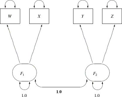
The only difference between the current path diagram in Figure 17.20 for the congeneric (one-factor) model and the preceding path diagram in Figure 17.17 for the full (two-factor) model is that the double-headed path that connects F1 and F2 is fixed to 1 in the current path diagram. Accordingly, you need to modify only slightly the preceding PROC CALIS specification to form the new model specification, as shown in the following statements:
proc calis data=lord;
   path
      W <--- F1,
      X <--- F1,
      Y <--- F2,
      Z <--- F2;
   pvar
      F1 = 1.0,
      F2 = 1.0,
      W X Y Z;
   pcov
      F1 F2 = 1.0;
run;
This specification sets the covariance between F1 and F2 to 1.0 in the PCOV statement. An annotated fit summary is displayed in Figure 17.21.
| Fit Summary | |
|---|---|
| Chi-Square | 36.2095 |
| Chi-Square DF | 2 |
| Pr > Chi-Square | <.0001 |
| Standardized RMSR (SRMSR) | 0.0277 |
| Adjusted GFI (AGFI) | 0.8570 |
| RMSEA Estimate | 0.1625 |
| Bentler Comparative Fit Index | 0.9766 |
The chi-square value is 36.2095 ( = 2, < 0.0001). This indicates that you can reject the hypothesized model at the 0.01  -level. The standardized root mean square error (SRMSR) is 0.0277, which indicates a good fit. Bentler’s comparative fit index is 0.9766, which is also a good model fit. However, the adjusted GFI (AGFI) is 0.8570, which is not very impressive. Also, the RMSEA value is 0.1625, which is too large to be an acceptable model. Therefore, the congeneric model might not be the one you want to use.
The estimation results are displayed in Figure 17.22. Because the model does not fit well, the corresponding estimation results are not interpreted.
| PATH List | ||||||
|---|---|---|---|---|---|---|
| Path | Parameter | Estimate | Standard Error |
t Value | ||
| W | <--- | F1 | _Parm1 | 7.10470 | 0.32177 | 22.08012 |
| X | <--- | F1 | _Parm2 | 7.26908 | 0.31826 | 22.83973 |
| Y | <--- | F2 | _Parm3 | 8.37344 | 0.32542 | 25.73143 |
| Z | <--- | F2 | _Parm4 | 8.51060 | 0.32409 | 26.26002 |
| Variance Parameters | |||||
|---|---|---|---|---|---|
| Variance Type |
Variable | Parameter | Estimate | Standard Error |
t Value |
| Exogenous | F1 | 1.00000 | |||
| F2 | 1.00000 | ||||
| Error | W | _Parm5 | 35.92111 | 2.41467 | 14.87619 |
| X | _Parm6 | 33.42373 | 2.31037 | 14.46684 | |
| Y | _Parm7 | 27.17043 | 2.24621 | 12.09613 | |
| Z | _Parm8 | 25.38887 | 2.20837 | 11.49664 | |
| Covariances Among Exogenous Variables | ||||
|---|---|---|---|---|
| Var1 | Var2 | Estimate | Standard Error |
t Value |
| F1 | F2 | 1.00000 | ||
Perhaps a more natural way to specify the model under hypothesis is to use only one factor in the PATH model, as shown in the following statements:
proc calis data=lord;
   path
      W <--- F1,
      X <--- F1,
      Y <--- F1,
      Z <--- F1;
   pvar
      F1 = 1.0,
      W X Y Z;
run;
This produces essentially the same results as the specification with two factors that have perfect correlation.
H2: Two-Factor Model with Parallel Tests for Lord Data
The path diagram for the two-factor model with parallel tests is shown in Figure 17.23.
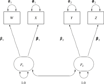
The hypothesis requires that variables or tests under each factor are "interchangeable." In terms of the measurement model, several pairs of parameters must be constrained to have equal estimates. That is, under the parallel-test model W and X should have the same effect or path coefficient  from their common factor F1, and they should also have the same measurement error variance
  . Similarly, Y and Z should have the same effect or path coefficient
  from their common factor F2, and they should also have the same measurement error variance
  . These constraints are labeled in Figure 17.23.
You can impose each of these equality constraints by giving the same name for the parameters involved in the PATH model specification. The following statements specify the path diagram in Figure 17.23:
proc calis data=lord;
   path
      W <--- F1   = beta1,
      X <--- F1   = beta1,
      Y <--- F2   = beta2,
      Z <--- F2   = beta2;
   pvar
      F1  = 1.0,
      F2  = 1.0,
      W X = 2 * theta1,
      Y Z = 2 * theta2;
   pcov
      F1 F2;
run;
Note that the specification 2*theta1 in the PVAR statement means that theta1 is specified twice for the error variances of the two variables W and X. Similarly for the specification 2*theta2. An annotated fit summary is displayed in Figure 17.24.
| Fit Summary | |
|---|---|
| Chi-Square | 1.9335 |
| Chi-Square DF | 5 |
| Pr > Chi-Square | 0.8583 |
| Standardized RMSR (SRMSR) | 0.0076 |
| Adjusted GFI (AGFI) | 0.9970 |
| RMSEA Estimate | 0.0000 |
| Bentler Comparative Fit Index | 1.0000 |
The chi-square value is 1.9335 (=5, =0.8583). This indicates that you cannot reject the hypothesized model H2. The standardized root mean square error (SRMSR) is 0.0076, which indicates a very good fit. Bentler’s comparative fit index is 1.0000. The adjusted GFI (AGFI) is 0.9970, and the RMSEA is close to zero. All results indicate that this is a good model for the data.
The estimation results are displayed in Figure 17.25.
| PATH List | ||||||
|---|---|---|---|---|---|---|
| Path | Parameter | Estimate | Standard Error |
t Value | ||
| W | <--- | F1 | beta1 | 7.60099 | 0.26844 | 28.31580 |
| X | <--- | F1 | beta1 | 7.60099 | 0.26844 | 28.31580 |
| Y | <--- | F2 | beta2 | 8.59186 | 0.27967 | 30.72146 |
| Z | <--- | F2 | beta2 | 8.59186 | 0.27967 | 30.72146 |
| Variance Parameters | |||||
|---|---|---|---|---|---|
| Variance Type |
Variable | Parameter | Estimate | Standard Error |
t Value |
| Exogenous | F1 | 1.00000 | |||
| F2 | 1.00000 | ||||
| Error | W | theta1 | 28.55545 | 1.58641 | 18.00000 |
| X | theta1 | 28.55545 | 1.58641 | 18.00000 | |
| Y | theta2 | 23.73200 | 1.31844 | 18.00000 | |
| Z | theta2 | 23.73200 | 1.31844 | 18.00000 | |
| Covariances Among Exogenous Variables | |||||
|---|---|---|---|---|---|
| Var1 | Var2 | Parameter | Estimate | Standard Error |
t Value |
| F1 | F2 | _Parm1 | 0.89864 | 0.01865 | 48.18011 |
Notice that because you explicitly specify the parameter names for the path coefficients (that is, beta1 and beta2), they are used in the output shown in Figure 17.25. The correlation between F1 and F2 is 0.8987, which is a very high correlation that suggests F1 and F2 might have been the same factor in the population. The next section sets this value to one so that the current model becomes a one-factor model with parallel tests.
H1: One-Factor Model with Parallel Tests for Lord Data
The path diagram for the one-factor model with parallel tests is shown in Figure 17.26.
The hypothesis differs from in that F1 and F2 have a perfect correlation in . This is indicated by the fixed value 1.0 for the double-headed path that connects F1 and F2 in Figure 17.26. Again, you need only minimal modification of the preceding specification for to specify the path diagram in Figure 17.26, as shown in the following statements:
proc calis data=lord;
   path
      W <--- F1   = beta1,
      X <--- F1   = beta1,
      Y <--- F2   = beta2,
      Z <--- F2   = beta2;
   pvar
      F1  = 1.0,
      F2  = 1.0,
      W X = 2 * theta1,
      Y Z = 2 * theta2;
   pcov
      F1 F2 = 1.0;
run;
The only modification of the preceding specification is in the PCOV statement, where you put a constant 1 for the covariance between F1 and F2. An annotated fit summary is displayed in Figure 17.27.
| Fit Summary | |
|---|---|
| Chi-Square | 37.3337 |
| Chi-Square DF | 6 |
| Pr > Chi-Square | <.0001 |
| Standardized RMSR (SRMSR) | 0.0286 |
| Adjusted GFI (AGFI) | 0.9509 |
| RMSEA Estimate | 0.0898 |
| Bentler Comparative Fit Index | 0.9785 |
The chi-square value is 37.3337 (=6, <0.0001). This indicates that you can reject the hypothesized model H1 at the 0.01 -level. The standardized root mean square error (SRMSR) is 0.0286, the adjusted GFI (AGFI) is 0.9509, and Bentler’s comparative fit index is 0.9785. All these indicate good model fit. However, the RMSEA is 0.0898, which does not support an acceptable model for the data.
The estimation results are displayed in Figure 17.28.
| PATH List | ||||||
|---|---|---|---|---|---|---|
| Path | Parameter | Estimate | Standard Error |
t Value | ||
| W | <--- | F1 | beta1 | 7.18623 | 0.26598 | 27.01802 |
| X | <--- | F1 | beta1 | 7.18623 | 0.26598 | 27.01802 |
| Y | <--- | F2 | beta2 | 8.44198 | 0.28000 | 30.14943 |
| Z | <--- | F2 | beta2 | 8.44198 | 0.28000 | 30.14943 |
| Variance Parameters | |||||
|---|---|---|---|---|---|
| Variance Type |
Variable | Parameter | Estimate | Standard Error |
t Value |
| Exogenous | F1 | 1.00000 | |||
| F2 | 1.00000 | ||||
| Error | W | theta1 | 34.68865 | 1.64634 | 21.07010 |
| X | theta1 | 34.68865 | 1.64634 | 21.07010 | |
| Y | theta2 | 26.28513 | 1.39955 | 18.78119 | |
| Z | theta2 | 26.28513 | 1.39955 | 18.78119 | |
| Covariances Among Exogenous Variables | ||||
|---|---|---|---|---|
| Var1 | Var2 | Estimate | Standard Error |
t Value |
| F1 | F2 | 1.00000 | ||
The goodness-of-fit tests for the four hypotheses are summarized in the following table.
Number of |
Degrees of |
||||
|---|---|---|---|---|---|
Hypothesis |
Parameters |
|
Freedom |
p-value |
|
|
4 |
37.33 |
6 |
< .0001 |
1.0 |
|
5 |
1.93 |
5 |
0.8583 |
0.8986 |
|
8 |
36.21 |
2 |
< .0001 |
1.0 |
|
9 |
0.70 |
1 |
0.4018 |
0.8986 |


Recall that the estimates of for and are almost identical, about 0.90, indicating that the speeded and unspeeded tests are measuring almost the same latent variable. However, when was set to 1 in and (both one-factor models), both hypotheses were rejected. Hypotheses and (both two-factor models) seem to be consistent with the data. Since is obtained by adding four constraints (for the requirement of parallel tests) to (the full model), you can test versus by computing the differences of the chi-square statistics and their degrees of freedom, yielding a chi-square of 1.23 with four degrees of freedom, which is obviously not significant. In a sense, the chi-square difference test means that representing the data by would not be significantly worse than representing the data by . In addition, because offers a more precise description of the data (with the assumption of parallel tests) than , it should be chosen because of its simplicity. In conclusion, the two-factor model with parallel tests provides the best explanation of the data.