The GLM Procedure
-
Overview

-
Getting Started
-
Syntax
-
Details
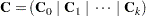
Statistical Assumptions for Using PROC GLM Specification of Effects Using PROC GLM Interactively Parameterization of PROC GLM Models Hypothesis Testing in PROC GLM Effect Size Measures for F Tests in GLM Absorption Specification of ESTIMATE Expressions Comparing Groups Multivariate Analysis of Variance Repeated Measures Analysis of Variance Random-Effects Analysis Missing Values Computational Resources Computational Method Output Data Sets Displayed Output ODS Table Names ODS Graphics
-
Examples
Randomized Complete Blocks with Means Comparisons and Contrasts Regression with Mileage Data Unbalanced ANOVA for Two-Way Design with Interaction Analysis of Covariance Three-Way Analysis of Variance with Contrasts Multivariate Analysis of Variance Repeated Measures Analysis of Variance Mixed Model Analysis of Variance with the RANDOM Statement Analyzing a Doubly Multivariate Repeated Measures Design Testing for Equal Group Variances Analysis of a Screening Design
- References
| Random-Effects Analysis |
When some model effects are random (that is, assumed to be sampled from a normal population of effects), you can specify these effects in the RANDOM statement in order to compute the expected values of mean squares for various model effects and contrasts and, optionally, to perform random-effects analysis of variance tests.
PROC GLM versus PROC MIXED for Random-Effects Analysis
Other SAS procedures that can be used to analyze models with random effects include the MIXED and VARCOMP procedures. Note that, for these procedures, the random-effects specification is an integral part of the model, affecting how both random and fixed effects are fit; for PROC GLM, the random effects are treated in a post hoc fashion after the complete fixed-effect model is fit. This distinction affects other features in the GLM procedure, such as the results of the LSMEANS and ESTIMATE statements. These features assume that all effects are fixed, so that all tests and estimability checks for these statements are based on a fixed-effects model, even when you use a RANDOM statement. Standard errors for estimates and LS-means based on the fixed-effects model might be significantly smaller than those based on a true random-effects model; in fact, some functions that are estimable under a true random-effects model might not even be estimable under the fixed-effects model. Therefore, you should use the MIXED procedure to compute tests involving these features that take the random effects into account; see Chapter 58, The MIXED Procedure, for more information.
Note that, for balanced data, the test statistics computed when you specify the TEST option in the RANDOM statement have an exact  distribution only when the design is balanced; for unbalanced designs, the
  values for the F tests are approximate. For balanced data, the values obtained by PROC GLM and PROC MIXED agree; for unbalanced data, they usually do not.
Computation of Expected Mean Squares for Random Effects
The RANDOM statement in PROC GLM declares one or more effects in the model to be random rather than fixed. By default, PROC GLM displays the coefficients of the expected mean squares for all terms in the model. In addition, when you specify the TEST option in the RANDOM statement, the procedure determines what tests are appropriate and provides ratios and probabilities for these tests.
The expected mean squares are computed as follows. Consider the model
 |
where  represents the fixed effects and
  represent the random effects. Random effects are assumed to be normally and independently distributed. For any
  in the row space of
  , the expected value of the sum of squares for
  is
is
 |
where  is of the same dimensions as and is partitioned as the
  matrix. In other words,
 |
Furthermore,  , where
  is the inverse of the lower triangular Cholesky decomposition matrix of
  . SSQ(
 ) is defined as tr
 .
.
For the model in the following MODEL statement
model Y=A B(A) C A*C;
random B(A);
with B(A) declared as random, the expected mean square of each effect is displayed as
 |
If any fixed effects appear in the expected mean square of an effect, the letter Q followed by the list of fixed effects in the expected value is displayed. The actual numeric values of the quadratic form ( matrix) can be displayed using the Q option.
To determine appropriate means squares for testing the effects in the model, the TEST option in the RANDOM statement performs the following steps:
First, it forms a matrix of coefficients of the expected mean squares of those effects that were declared to be random.
-
Next, for each effect in the model, it determines the combination of these expected mean squares that produce an expectation that includes all the terms in the expected mean square of the effect of interest except the one corresponding to the effect of interest. For example, if the expected mean square of an effect A*B is

PROC GLM determines the combination of other expected mean squares in the model that has expectation
If the preceding criterion is met by the expected mean square of a single effect in the model (as is often the case in balanced designs), the
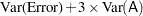
test is formed directly. In this case, the mean square of the effect of interest is used as the numerator, the mean square of the single effect with an expected mean square that satisfies the criterion is used as the denominator, and the degrees of freedom for the test are simply the usual model degrees of freedom. When more than one mean square must be combined to achieve the appropriate expectation, an approximation is employed to determine the appropriate degrees of freedom (Satterthwaite; 1946). When effects other than the effect of interest are listed after the Q in the output, tests of hypotheses involving the effect of interest are not valid unless all other fixed effects involved in it are assumed to be zero. When tests such as these are performed by using the TEST option in the RANDOM statement, a note is displayed reminding you that further assumptions are necessary for the validity of these tests. Remember that although the tests are not valid unless these assumptions are made, this does not provide a basis for these assumptions to be true. The particulars of a given experiment must be examined to determine whether the assumption is reasonable.
See Goodnight and Speed (1978), Milliken and Johnson (1984, Chapters 22 and 23), and Hocking (1985) for further theoretical discussion.
Sum-to-Zero Assumptions
The formulation and parameterization of the expected mean squares for random effects in mixed models are ongoing items of controversy in the statistical literature. Confusion arises over whether or not to assume that terms involving fixed effects sum to zero. Cornfield and Tukey (1956), Winer (1971), and others assume that they do sum to zero; Searle (1971), Hocking (1973), and others (including PROC GLM) do not.
Different assumptions about these sum-to-zero constraints can lead to different expected mean squares for certain terms, and hence to different F and values.
For arguments in favor of not assuming that terms involving fixed effects sum to zero, see Section 9.7 of Searle (1971) and Sections 1 and 4 of McLean, Sanders, and Stroup (1991). Other references are Hartley and Searle (1969) and Searle, Casella, and McCulloch (1992).
Computing Type I, II, and IV Expected Mean Squares
When you use the RANDOM statement, by default the GLM procedure produces the Type III expected mean squares for model effects and for contrasts specified before the RANDOM statement. In order to obtain expected values for other types of mean squares, you need to specify which types of mean squares are of interest in the MODEL statement. For example, in order to obtain the Type IV expected mean squares for effects in the RANDOM and CONTRAST statements, specify the SS4 option in the MODEL statement. If you want both Type III and Type IV expected mean squares, specify both the SS3 and SS4 options in the MODEL statement. Since the estimable function basis is not automatically calculated for Type I and Type II SS, the E1 (for Type I) or E2 (for Type II) option must be specified in the MODEL statement in order for the RANDOM statement to produce the expected mean squares for the Type I or Type II sums of squares. Note that it is important to list the fixed effects first in the MODEL statement when requesting the Type I expected mean squares.
For example, suppose you have a two-way design with factors A and B in which the main effect for B and the interaction are random. In order to compute the Type III expected mean squares (in addition to the fixed-effect analysis), you can use the following statements:
proc glm;
   class A B;
   model Y = A B A*B;
   random B A*B;
run;
Suppose you use the SS4 option in the MODEL statement, as follows:
proc glm;
   class A B;
   model Y = A B A*B / ss4;
   random B A*B;
run;
Then only the Type IV expected mean squares are computed (as well as the Type IV fixed-effect tests). For the Type I expected mean squares, you can use the following statements:
proc glm;
   class A B;
   model Y = A B A*B / e1;
   random B A*B;
run;
For each of these cases, in order to perform random-effect analysis of variance tests for each effect specified in the model, you need to specify the TEST option in the RANDOM statement, as follows:
proc glm;
   class A B;
   model Y = A B A*B;
   random B A*B / test;
run;
The GLM procedure automatically determines the appropriate error term for each test, based on the expected mean squares.