The GLM Procedure
-
Overview

-
Getting Started
-
Syntax
-
Details
Statistical Assumptions for Using PROC GLM Specification of Effects Using PROC GLM Interactively Parameterization of PROC GLM Models Hypothesis Testing in PROC GLM Effect Size Measures for F Tests in GLM Absorption Specification of ESTIMATE Expressions Comparing Groups Multivariate Analysis of Variance Repeated Measures Analysis of Variance Random-Effects Analysis Missing Values Computational Resources Computational Method Output Data Sets Displayed Output ODS Table Names ODS Graphics
-
Examples
Randomized Complete Blocks with Means Comparisons and Contrasts Regression with Mileage Data Unbalanced ANOVA for Two-Way Design with Interaction Analysis of Covariance Three-Way Analysis of Variance with Contrasts Multivariate Analysis of Variance Repeated Measures Analysis of Variance Mixed Model Analysis of Variance with the RANDOM Statement Analyzing a Doubly Multivariate Repeated Measures Design Testing for Equal Group Variances Analysis of a Screening Design
- References
| PROC GLM for Quadratic Least Squares Regression |
In polynomial regression, the values of a dependent variable (also called a response variable) are described or predicted in terms of polynomial terms involving one or more independent or explanatory variables. An example of quadratic regression in PROC GLM follows. These data are taken from Draper and Smith (1966, p. 57). Thirteen specimens of 90/10 Cu-Ni alloys are tested in a corrosion-wheel setup in order to examine corrosion. Each specimen has a certain iron content. The wheel is rotated in salt sea water at 30 ft/sec for 60 days. Weight loss is used to quantify the corrosion. The fe variable represents the iron content, and the loss variable denotes the weight loss in milligrams/square decimeter/day in the following DATA step.
title 'Regression in PROC GLM';
data iron;
   input fe loss @@;
   datalines;
0.01 127.6   0.48 124.0   0.71 110.8   0.95 103.9
1.19 101.5   0.01 130.1   0.48 122.0   1.44  92.3
0.71 113.1   1.96  83.7   0.01 128.0   1.44  91.4
1.96  86.2
;
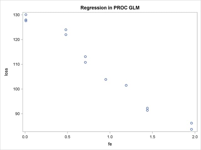
The SGSCATTER procedure is used in the following statements to request a scatter plot of the response variable versus the independent variable.
ods graphics on;
proc sgscatter data=iron;
   plot loss*fe;
run;
ods graphics off;
The plot in Figure 41.4 displays a strong negative relationship between iron content and corrosion resistance, but it is not clear whether there is curvature in this relationship.
The following statements fit a quadratic regression model to the data. This enables you to estimate the linear relationship between iron content and corrosion resistance and to test for the presence of a quadratic component. The intercept is automatically fit unless the NOINT option is specified.
proc glm data=iron;
   model loss=fe fe*fe;
run;
The CLASS statement is omitted because a regression line is being fitted. Unlike PROC REG, PROC GLM allows polynomial terms in the MODEL statement.
PROC GLM first displays preliminary information, shown in Figure 41.5, telling you that the GLM procedure has been invoked and stating the number of observations in the data set. If the model involves classification variables, they are also listed here, along with their levels.
| Regression in PROC GLM |
| Number of Observations Read | 13 |
|---|---|
| Number of Observations Used | 13 |
Figure 41.6 shows the overall ANOVA table and some simple statistics. The degrees of freedom can be used to check that the model is correct and that the data have been read correctly. The Model degrees of freedom for a regression is the number of parameters in the model minus 1. You are fitting a model with three parameters in this case,
 |
 |
 |
so the degrees of freedom are  . The Corrected Total degrees of freedom are always one less than the number of observations used in the analysis.
| Regression in PROC GLM |
| Source | DF | Sum of Squares | Mean Square | F Value | Pr > F |
|---|---|---|---|---|---|
| Model | 2 | 3296.530589 | 1648.265295 | 164.68 | <.0001 |
| Error | 10 | 100.086334 | 10.008633 | ||
| Corrected Total | 12 | 3396.616923 |
| R-Square | Coeff Var | Root MSE | loss Mean |
|---|---|---|---|
| 0.970534 | 2.907348 | 3.163642 | 108.8154 |
The  indicates that the model accounts for 97% of the variation in LOSS. The coefficient of variation (Coeff Var), Root MSE (Mean Square for Error), and mean of the dependent variable are also listed.
The overall  test is significant
  , indicating that the model as a whole accounts for a significant amount of the variation in LOSS. Thus, it is appropriate to proceed to testing the effects.
Figure 41.7 contains tests of effects and parameter estimates. The latter are displayed by default when the model contains only continuous variables.
| Source | DF | Type I SS | Mean Square | F Value | Pr > F |
|---|---|---|---|---|---|
| fe | 1 | 3293.766690 | 3293.766690 | 329.09 | <.0001 |
| fe*fe | 1 | 2.763899 | 2.763899 | 0.28 | 0.6107 |
| Source | DF | Type III SS | Mean Square | F Value | Pr > F |
|---|---|---|---|---|---|
| fe | 1 | 356.7572421 | 356.7572421 | 35.64 | 0.0001 |
| fe*fe | 1 | 2.7638994 | 2.7638994 | 0.28 | 0.6107 |
| Parameter | Estimate | Standard Error | t Value | Pr > |t| |
|---|---|---|---|---|
| Intercept | 130.3199337 | 1.77096213 | 73.59 | <.0001 |
| fe | -26.2203900 | 4.39177557 | -5.97 | 0.0001 |
| fe*fe | 1.1552018 | 2.19828568 | 0.53 | 0.6107 |
The  tests provided are equivalent to the Type III tests. The quadratic term is not significant
  and thus can be removed from the model; the linear term is significant
  . This suggests that there is indeed a straight-line relationship between loss and fe.
Finally, if ODS Graphics is enabled, PROC GLM also displays by default a scatter plot of the original data, as in Figure 41.4, with the quadratic fit overlaid. The following statements, which are the same as the previous analysis but with ODS Graphics enabled, additionally produce Figure 41.8.
ods graphics on;
proc glm data=iron;
   model loss=fe fe*fe;
run;
ods graphics off;
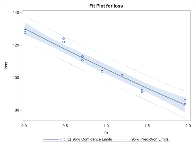
The insignificance of the quadratic term in the model is reflected in the fact that the fit is nearly linear.
Fitting the model without the quadratic term provides more accurate estimates for  and
and  . PROC GLM allows only one MODEL statement per invocation of the procedure, so the PROC GLM statement must be issued again. The following statements are used to fit the linear model.
proc glm data=iron;
   model loss=fe;
run;
Figure 41.9 displays the output produced by these statements. The linear term is still significant  . The estimated model is now
|
|
 |
| Regression in PROC GLM |
| Source | DF | Sum of Squares | Mean Square | F Value | Pr > F |
|---|---|---|---|---|---|
| Model | 1 | 3293.766690 | 3293.766690 | 352.27 | <.0001 |
| Error | 11 | 102.850233 | 9.350021 | ||
| Corrected Total | 12 | 3396.616923 |
| R-Square | Coeff Var | Root MSE | loss Mean |
|---|---|---|---|
| 0.969720 | 2.810063 | 3.057780 | 108.8154 |
| Source | DF | Type I SS | Mean Square | F Value | Pr > F |
|---|---|---|---|---|---|
| fe | 1 | 3293.766690 | 3293.766690 | 352.27 | <.0001 |
| Source | DF | Type III SS | Mean Square | F Value | Pr > F |
|---|---|---|---|---|---|
| fe | 1 | 3293.766690 | 3293.766690 | 352.27 | <.0001 |
| Parameter | Estimate | Standard Error | t Value | Pr > |t| |
|---|---|---|---|---|
| Intercept | 129.7865993 | 1.40273671 | 92.52 | <.0001 |
| fe | -24.0198934 | 1.27976715 | -18.77 | <.0001 |