The GLIMMIX Procedure
-
Overview

-
Getting Started
-
Syntax
PROC GLIMMIX Statement BY Statement CLASS Statement CONTRAST Statement COVTEST Statement EFFECT Statement ESTIMATE Statement FREQ Statement ID Statement LSMEANS Statement LSMESTIMATE Statement MODEL Statement NLOPTIONS Statement OUTPUT Statement PARMS Statement RANDOM Statement SLICE Statement STORE Statement WEIGHT Statement Programming Statements User-Defined Link or Variance Function
-
Details
Generalized Linear Models Theory Generalized Linear Mixed Models Theory GLM Mode or GLMM Mode Statistical Inference for Covariance Parameters Satterthwaite Degrees of Freedom Approximation Empirical Covariance (Sandwich) Estimators Exploring and Comparing Covariance Matrices Processing by Subjects Radial Smoothing Based on Mixed Models Odds and Odds Ratio Estimation Parameterization of Generalized Linear Mixed Models Response-Level Ordering and Referencing Comparing the GLIMMIX and MIXED Procedures Singly or Doubly Iterative Fitting Default Estimation Techniques Default Output Notes on Output Statistics ODS Table Names ODS Graphics
-
Examples
Binomial Counts in Randomized Blocks Mating Experiment with Crossed Random Effects Smoothing Disease Rates; Standardized Mortality Ratios Quasi-likelihood Estimation for Proportions with Unknown Distribution Joint Modeling of Binary and Count Data Radial Smoothing of Repeated Measures Data Isotonic Contrasts for Ordered Alternatives Adjusted Covariance Matrices of Fixed Effects Testing Equality of Covariance and Correlation Matrices Multiple Trends Correspond to Multiple Extrema in Profile Likelihoods Maximum Likelihood in Proportional Odds Model with Random Effects Fitting a Marginal (GEE-Type) Model Response Surface Comparisons with Multiplicity Adjustments Generalized Poisson Mixed Model for Overdispersed Count Data Comparing Multiple B-Splines Diallel Experiment with Multimember Random Effects Linear Inference Based on Summary Data
- References
From Penalized Splines to Mixed Models
The connection between splines and mixed models arises from the similarity of the penalized spline fitting criterion to the minimization problem that yields the mixed model equations and solutions for  and
and  . This connection is made explicit in the following paragraphs. An important distinction between classical spline fitting and its mixed model smoothing variant, however, lies in the nature of the spline coefficients. Although they address similar minimization criteria, the solutions for the spline coefficients in the GLIMMIX procedure are the solutions of random effects, not fixed effects. Standard errors of predicted values, for example, account for this source of variation.
Consider the linearized mixed pseudo-model from the section The Pseudo-model, 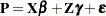 . One derivation of the mixed model equations, whose solutions are
  and
and  , is to maximize the joint density of
  with respect to and . This is not a true likelihood problem, because is not a parameter, but a random vector.
In the special case with  and
and  , the maximization of is equivalent to the minimization of
 |
Now consider a linear spline as in Ruppert, Wand, and Carroll (2003, p. 108),
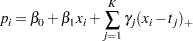 |
where the  denote the spline coefficients at knots
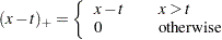
  . The truncated line function is defined as
 |
If you collect the intercept and regressor  into the matrix
  , and if you collect the truncated line functions into the
  matrix
  , then fitting the linear spline amounts to minimization of the penalized spline criterion
 |
where  is the smoothing parameter.
Because minimizing  with respect to and is equivalent to minimizing
  , both problems lead to the same solution, and
  is the smoothing parameter. The mixed model formulation of spline smoothing has the advantage that the smoothing parameter is selected "automatically." It is a function of the covariance parameter estimates, which, in turn, are estimated according to the method you specify with the METHOD= option in the PROC GLIMMIX statement.
To accommodate nonnormal responses and general link functions, the GLIMMIX procedure uses 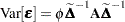 , where
  is the matrix of variance functions and
  is the diagonal matrix of mean derivatives defined earlier. The correspondence between spline smoothing and mixed modeling is then one between a weighted linear mixed model and a weighted spline. In other words, the minimization criterion that yields the estimates and solutions is then
 |
If you choose the TYPE=RSMOOTH covariance structure, PROC GLIMMIX chooses radial basis functions as the spline basis and transforms them to approximate a thin-plate spline as in Chapter 13.4 of Ruppert, Wand, and Carroll (2003). For computational expediency, the number of knots is chosen to be less than the number of data points. Ruppert, Wand, and Carroll (2003) recommend one knot per every four unique regressor values for one-dimensional smoothers. In the multivariate case, general recommendations are more difficult, because the optimal number and placement of knots depend on the spatial configuration of samples. Their recommendation for a bivariate smoother is one knot per four samples, but at least 20 and no more than 150 knots (Ruppert, Wand, and Carroll 2003, p. 257).
The magnitude of the variance component  depends on the metric of the random effects. For example, if you apply radial smoothing in time, the variance changes if you measure time in days or minutes. If the solution for the variance component is near zero, then a rescaling of the random effect data can help the optimization problem by moving the solution for the variance component away from the boundary of the parameter space.