The DISTANCE Procedure

| Creating a Distance Matrix as Input for a Subsequent Cluster Analysis |
The following example demonstrates how you can use the DISTANCE procedure to obtain a distance matrix that will be used as input to a subsequent clustering procedure.
The following data, originated by A. Weber and cited in Hand et al. (1994, p. 297), measure the amount of protein consumed for nine food groups in 25 European countries. The nine food groups are red meat (RedMeat), white meat (WhiteMeat), eggs (Eggs), milk (Milk), fish (Fish), cereal (Cereal), starch (Starch), nuts (Nuts), and fruits and vegetables (FruitVeg). Suppose you want to determine whether national figures in protein consumption can be used to determine certain types or categories of countries; specifically, you want to perform a cluster analysis to determine whether these 25 countries can be formed into groups suggested by the data.
The following DATA step creates the SAS data set Protein:
data Protein;
   input Country $14. RedMeat WhiteMeat Eggs Milk
                      Fish Cereal Starch Nuts FruitVeg;
   datalines;
Albania        10.1  1.4  0.5   8.9  0.2  42.3  0.6  5.5  1.7
Austria         8.9 14.0  4.3  19.9  2.1  28.0  3.6  1.3  4.3
Belgium        13.5  9.3  4.1  17.5  4.5  26.6  5.7  2.1  4.0
Bulgaria        7.8  6.0  1.6   8.3  1.2  56.7  1.1  3.7  4.2
Czechoslovakia  9.7 11.4  2.8  12.5  2.0  34.3  5.0  1.1  4.0
Denmark        10.6 10.8  3.7  25.0  9.9  21.9  4.8  0.7  2.4
E Germany       8.4 11.6  3.7  11.1  5.4  24.6  6.5  0.8  3.6
Finland         9.5  4.9  2.7  33.7  5.8  26.3  5.1  1.0  1.4
France         18.0  9.9  3.3  19.5  5.7  28.1  4.8  2.4  6.5
Greece         10.2  3.0  2.8  17.6  5.9  41.7  2.2  7.8  6.5
Hungary         5.3 12.4  2.9   9.7  0.3  40.1  4.0  5.4  4.2
Ireland        13.9 10.0  4.7  25.8  2.2  24.0  6.2  1.6  2.9
Italy           9.0  5.1  2.9  13.7  3.4  36.8  2.1  4.3  6.7
Netherlands     9.5 13.6  3.6  23.4  2.5  22.4  4.2  1.8  3.7
Norway          9.4  4.7  2.7  23.3  9.7  23.0  4.6  1.6  2.7
Poland          6.9 10.2  2.7  19.3  3.0  36.1  5.9  2.0  6.6
Portugal        6.2  3.7  1.1   4.9 14.2  27.0  5.9  4.7  7.9
Romania         6.2  6.3  1.5  11.1  1.0  49.6  3.1  5.3  2.8
Spain           7.1  3.4  3.1   8.6  7.0  29.2  5.7  5.9  7.2
Sweden          9.9  7.8  3.5   4.7  7.5  19.5  3.7  1.4  2.0
Switzerland    13.1 10.1  3.1  23.8  2.3  25.6  2.8  2.4  4.9
UK             17.4  5.7  4.7  20.6  4.3  24.3  4.7  3.4  3.3
USSR            9.3  4.6  2.1  16.6  3.0  43.6  6.4  3.4  2.9
W Germany      11.4 12.5  4.1  18.8  3.4  18.6  5.2  1.5  3.8
Yugoslavia      4.4  5.0  1.2   9.5  0.6  55.9  3.0  5.7  3.2
;
The data set Protein contains the character variable Country and the nine numeric variables representing the food groups. The $14. in the INPUT statement specifies that the variable Country has a length of 14.
The following statements create the distance matrix and display part of it:
title 'Protein Consumption in Europe';
proc distance data=Protein out=Dist method=Euclid;
   var interval(RedMeat--FruitVeg / std=Std);
   id Country;
run;
proc print data=Dist(obs=10);
   title2 'First 10 Observations in Output Data Set from PROC DISTANCE';
run;
title2;
An output SAS data set called Dist, which contains the distance matrix, is created through the OUT= option. The METHOD=EUCLID option requests that Euclidean distances (which is the default) should be computed and produces an output data set of TYPE=DISTANCE.1
The VAR statement lists the variables (RedMeat—FruitVeg) along with their measurement level to be used in the analysis. An interval level of measurement is assigned to those variables. Since variables with large variances tend to have more effect on the proximity measure than those with small variances, each variable is standardized by the STD method to have a mean of 0 and a standard deviation of 1. This is done by adding "/ STD=STD" at the end of the variables list.
The ID statement specifies that the variable Country should be copied to the OUT= data set and used to generate names for the distance variables. The distance variables in the output data set are named by the values in the ID variable, and the maximum length for the names of these variables is 14.
There are 25 observations in the input data set; therefore, the output data set Dist contains a 25-by-25 lower triangular matrix.
The PROC PRINT statement displays the first 10 observations in the output data set Dist as shown in Figure 33.1.
| Protein Consumption in Europe |
| First 10 Observations in Output Data Set from PROC DISTANCE |
| Obs | Country | Albania | Austria | Belgium | Bulgaria | Czechoslovakia | Denmark | E_Germany | Finland | France | Greece | Hungary | Ireland | Italy | Netherlands | Norway | Poland | Portugal | Romania | Spain | Sweden | Switzerland | UK | USSR | W_Germany | Yugoslavia |
|---|---|---|---|---|---|---|---|---|---|---|---|---|---|---|---|---|---|---|---|---|---|---|---|---|---|---|
| 1 | Albania | 0.00000 | . | . | . | . | . | . | . | . | . | . | . | . | . | . | . | . | . | . | . | . | . | . | . | . |
| 2 | Austria | 6.12388 | 0.00000 | . | . | . | . | . | . | . | . | . | . | . | . | . | . | . | . | . | . | . | . | . | . | . |
| 3 | Belgium | 5.94109 | 2.44987 | 0.00000 | . | . | . | . | . | . | . | . | . | . | . | . | . | . | . | . | . | . | . | . | . | . |
| 4 | Bulgaria | 2.76446 | 4.88331 | 5.22711 | 0.00000 | . | . | . | . | . | . | . | . | . | . | . | . | . | . | . | . | . | . | . | . | . |
| 5 | Czechoslovakia | 5.13959 | 2.11498 | 2.21330 | 3.94761 | 0.00000 | . | . | . | . | . | . | . | . | . | . | . | . | . | . | . | . | . | . | . | . |
| 6 | Denmark | 6.61002 | 3.01392 | 2.52541 | 6.00803 | 3.34049 | 0.00000 | . | . | . | . | . | . | . | . | . | . | . | . | . | . | . | . | . | . | . |
| 7 | E Germany | 6.39178 | 2.56341 | 2.10211 | 5.40824 | 1.87962 | 2.72112 | 0.00000 | . | . | . | . | . | . | . | . | . | . | . | . | . | . | . | . | . | . |
| 8 | Finland | 5.81458 | 4.04271 | 3.45779 | 5.74882 | 3.91378 | 2.61570 | 3.99426 | 0.00000 | . | . | . | . | . | . | . | . | . | . | . | . | . | . | . | . | . |
| 9 | France | 6.29601 | 3.58891 | 2.19329 | 5.54675 | 3.36011 | 3.65772 | 3.78184 | 4.56796 | 0.00000 | . | . | . | . | . | . | . | . | . | . | . | . | . | . | . | . |
| 10 | Greece | 4.24495 | 5.16330 | 4.69515 | 3.74849 | 4.86684 | 5.59084 | 5.61496 | 5.47453 | 4.54456 | 0 | . | . | . | . | . | . | . | . | . | . | . | . | . | . | . |
The following statements produce the dendrogram in Figure 33.2:
ods graphics on;

proc cluster data=Dist method=Ward plots=dendrogram(height=rsq);
   id Country;
run;
The CLUSTER procedure performs a Ward’s minimum-variance cluster analysis based on the distance matrix created by PROC DISTANCE. PROC CLUSTER, along with ODS Graphics, produces the dendrogram shown in Figure 33.2. The option PLOTS=DENDROGRAM(HEIGHT=RSQ) specifies the squared multiple correlation as the height variable in the dendrogram.
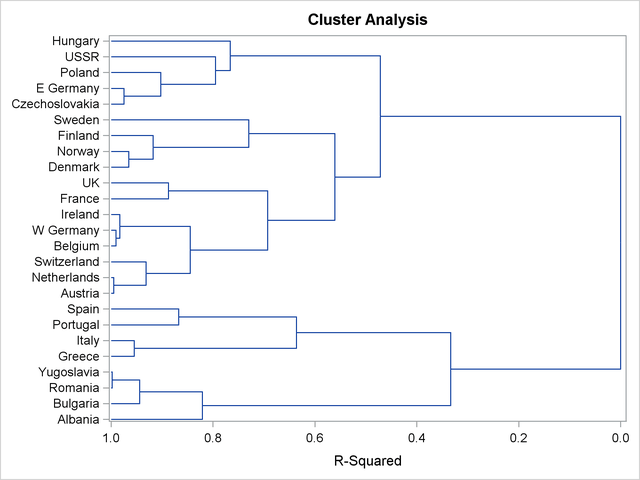
After inspecting the dendrogram in Figure 33.2, you will see that when the countries are grouped into six clusters, the proportion of variance accounted for by these clusters is slightly less than 70% (69.3%). The 25 countries are clustered as follows:
Balkan countries: Albania, Bulgaria, Romania, and Yugoslavia
Mediterranean countries: Greece and Italy
Iberian countries: Portugal and Spain
Western European countries: Austria, Netherlands, Switzerland, Belgium, former West Germany, Ireland, France, and U.K.
Scandinavian countries: Denmark, Norway, Finland, and Sweden
Eastern European countries: former Czechoslovakia, former East Germany, Poland, former U.S.S.R., and Hungary
Footnotes
- Data set types do not persist when you copy or modify a data set. You must specify the TYPE= data set option for the new data set. See the METHOD= and OUT= options for more information about data set types.