| The QUANTREG Procedure |
Example 73.5 Quantile Polynomial Regression for Salary Data
This example uses the data set from a university union survey of salaries of professors in 1991. The survey covered departments in U.S. colleges and universities that list programs in statistics. The goal here is to examine the relationship between faculty salaries and years of service.
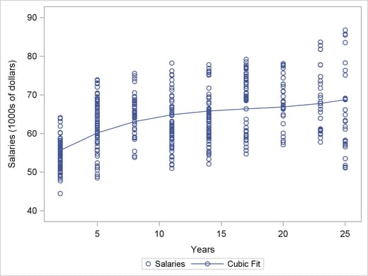
The data include salaries and years of service for 459 professors. The scatter plot in Output 73.5.1 shows that the relationship is not linear, and a quadratic or cubic regression curve is appropriate. Output 73.5.1 shows a cubic curve.
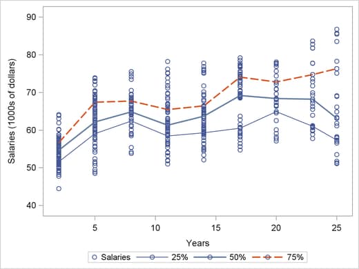
The curve in Output 73.5.1 does not adequately describe the conditional salary distributions and how they change with length of service. Output 73.5.2 shows the 25th, 50th, and 75th percentiles for each number of years, which gives a better picture of the conditional distributions.
data salary;
  label salaries='Salaries (1000s of dollars)'
        years   ='Years';
  input salaries years @@;
datalines;
54.94   2  58.24   2  58.11   2  52.23   2  52.98    2  57.62    2
44.48   2  57.22   2  54.24   2  54.79   2  56.42    2  61.90    2
63.90   2  64.10   2  47.77   2  54.86   2  49.31    2  53.37    2

   ... more lines ...

85.72  25  64.87  25  51.76  25  51.11  25  51.31   25  78.28   25
57.91  25  86.78  25  58.27  25  56.56  25  76.33   25  61.83   25
69.13  25  63.15  25  66.13  25
;
These descriptive percentiles do not clearly show trends with length of service. The following statements use the QUANTREG procedure to obtain a smooth version by using polynomial quantile regression. The results are shown in Output 73.5.3 and Output 73.5.4.
ods graphics on;

proc quantreg data=salary ci=sparsity;
   model salaries = years years*years years*years*years
                     /quantile=0.25 0.5 0.75
                     plot=fitplot(showlimits);
run;

ods graphics off;
Output 73.5.3 shows the regression coefficients for the three quantiles.
| Parameter Estimates | |||||||
|---|---|---|---|---|---|---|---|
| Parameter | DF | Estimate | Standard Error | 95% Confidence Limits | t Value | Pr > |t| | |
| Intercept | 1 | 48.2509 | 1.3484 | 45.6011 | 50.9007 | 35.78 | <.0001 |
| years | 1 | 2.2234 | 0.5455 | 1.1514 | 3.2953 | 4.08 | <.0001 |
| years*years | 1 | -0.1292 | 0.0500 | -0.2275 | -0.0308 | -2.58 | 0.0101 |
| years*years*years | 1 | 0.0024 | 0.0013 | -0.0001 | 0.0049 | 1.86 | 0.0634 |
| Parameter Estimates | |||||||
|---|---|---|---|---|---|---|---|
| Parameter | DF | Estimate | Standard Error | 95% Confidence Limits | t Value | Pr > |t| | |
| Intercept | 1 | 50.2512 | 1.2812 | 47.7334 | 52.7690 | 39.22 | <.0001 |
| years | 1 | 2.7173 | 0.5947 | 1.5485 | 3.8860 | 4.57 | <.0001 |
| years*years | 1 | -0.1632 | 0.0632 | -0.2873 | -0.0390 | -2.58 | 0.0101 |
| years*years*years | 1 | 0.0034 | 0.0018 | -0.0002 | 0.0070 | 1.85 | 0.0647 |
| Parameter Estimates | |||||||
|---|---|---|---|---|---|---|---|
| Parameter | DF | Estimate | Standard Error | 95% Confidence Limits | t Value | Pr > |t| | |
| Intercept | 1 | 51.0298 | 1.5886 | 47.9078 | 54.1517 | 32.12 | <.0001 |
| years | 1 | 3.6513 | 0.7594 | 2.1590 | 5.1436 | 4.81 | <.0001 |
| years*years | 1 | -0.2390 | 0.0764 | -0.3892 | -0.0888 | -3.13 | 0.0019 |
| years*years*years | 1 | 0.0055 | 0.0021 | 0.0013 | 0.0096 | 2.60 | 0.0098 |
Output 73.5.4 displays the three cubic percentile curves with 95% confidence limits.
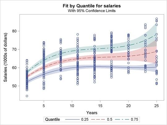
The three curves show that salary dispersion increases gradually with length of service. After 15 years, a salary over $70,000 is relatively high, while a salary less than $60,000 is relatively low. Note that percentile curves of this type are useful in medical science as reference curves; see Yu, Lu, and Stabder (2003).
Copyright © SAS Institute, Inc. All Rights Reserved.