| The QUANTREG Procedure |
Example 73.4 Nonparametric Quantile Regression for Ozone Levels
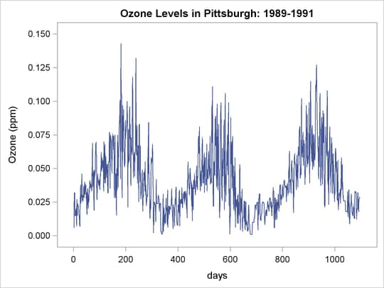
Tracing seasonal trends in the level of tropospheric ozone is essential for predicting high-level periods, observing long-term trends, and discovering potential changes in pollution. Traditional methods for modeling seasonal effects are based on the conditional mean of ozone concentration; however, the upper conditional quantiles are more critical from a public health perspective. In this example, the QUANTREG procedure fits conditional quantile curves for seasonal effects by using nonparametric quantile regression with cubic B-splines.
The data used here are from Chock, Winkler, and Chen (2000), who studied the association between daily mortality and ambient air pollutant concentrations in Pittsburgh, Pennsylvania. The data set ozone contains the following two variables: ozone (daily-maximum one-hour ozone concentration (ppm)) and days (index of 1,095 days (3 years)).
data ozone;
  days = _n_;
  input ozone @@;
datalines;
0.0060 0.0060 0.0320 0.0320 0.0320 0.0150 0.0150 0.0150 0.0200 0.0200
0.0160 0.0070 0.0270 0.0160 0.0150 0.0240 0.0220 0.0220 0.0220 0.0185
0.0150 0.0150 0.0110 0.0070 0.0070 0.0240 0.0380 0.0240 0.0265 0.0290

   ... more lines ...

0.0220 0.0210 0.0210 0.0130 0.0130 0.0130 0.0330 0.0330 0.0330 0.0325
0.0320 0.0320 0.0320 0.0120 0.0200 0.0200 0.0200 0.0320 0.0320 0.0250
0.0180 0.0180 0.0270 0.0270 0.0290
;
Output 73.4.1, which displays the time series plot of ozone concentration for the three years, shows a clear seasonal pattern.
In this example, cubic B-splines are used to fit the seasonal effect. These splines are generated with 11 knots, which split the 3 years into 12 seasons. The following statements create the spline basis and fit multiple quantile regression spline curves:
ods graphics on;

proc quantreg data=ozone algorithm=smooth plot=fitplot(nodata);
   effect sp = spline( days / knotmethod = list
          (90 182 272 365 455 547 637 730 820 912 1002) );
   model ozone = sp / quantile = 0.5 0.75 0.90 0.95 seed=1268;
run;

ods graphics off;
The EFFECT statement creates spline bases for the variable days. The KNOTMETHOD=LIST option provides all internal knots for these bases. Cubic spline bases are generated by default. These bases are treated as components of the spline effect sp, which is used in the MODEL statement. Spline fits for four quantiles are requested with the QUANTILE= option.
When you enable ODS Graphics, the QUANTREG procedure automatically generates a fit plot, which includes all fitted curves.
Output 73.4.2 displays these curves obtained with the QUANTREG procedure. The curves show that peak ozone levels occur in the summer. For the three years (1989–1991), the median curve (labeled 50 ) does not cross the 0.08 ppm line, which is the 1997 EPA 8-hour standard. The median curve and the 75 curve show a drop for the ozone concentration levels in 1990. However, with the 90 and 95 curves, peak ozone levels tend to increase. This indicates that there might have been more days with low ozone concentration in 1990, but the top 10 and 5 tend to have higher ozone concentration levels.
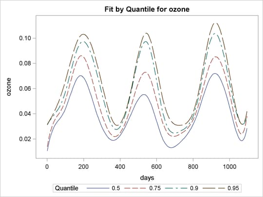
The quantile curves also show that high ozone concentration in 1989 had a longer duration than in 1990 and 1991. This is indicated by the wider spread of the quantile curves in 1989.
Copyright © SAS Institute, Inc. All Rights Reserved.