| The MCMC Procedure |
Example 52.5 Random-Effects Models
This example illustrates how you can use PROC MCMC to fit random effects models. In the example Mixed-Effects Model in Getting Started: MCMC Procedure, you already saw PROC MCMC fit a linear random effects model. There are two more examples in this section. One is a logistic random effects model, and the second one is a nonlinear Poisson regression random effects model. In addition, this section illustrates how to construct prior distributions that depend on input data set variables. Such prior distributions appear frequently in random effects model, especially in cases of hierarchical centering. Although you can use PROC MCMC to analyze random effects models, you might want to first consider some other SAS procedures. For example, you can use PROC MIXED (see Chapter 56, The MIXED Procedure ) to analyze linear mixed effects models, PROC NLMIXED (see Chapter 61, The NLMIXED Procedure ) for nonlinear mixed effects models, and PROC GLIMMIX (see Chapter 38, The GLIMMIX Procedure ) for generalized linear mixed effects models. In addition, a sampling-based Bayesian analysis is available in the MIXED procedure through the PRIOR statement (see PRIOR Statement).
Logistic Regression Random-Effects Model
This example shows how to fit a logistic random-effects model in PROC MCMC. The data are taken from Crowder (1978). The seeds data set is a  factorial layout, with two types of seeds, O. aegyptiaca 75 and O. aegyptiaca 73, and two root extracts, bean and cucumber. You observe r, which is the number of germinated seeds, and n, which is the total number of seeds. The independent variables are seed and extract.
The following statements create the data set:
title 'Logistic Regression Random-Effects Model';
data seeds;
   input r n seed extract @@;
   ind = _N_;
   datalines;
10  39  0  0    23  62  0  0    23  81  0  0    26  51  0  0
17  39  0  0     5   6  0  1    53  74  0  1    55  72  0  1
32  51  0  1    46  79  0  1    10  13  0  1     8  16  1  0
10  30  1  0     8  28  1  0    23  45  1  0     0   4  1  0
 3  12  1  1    22  41  1  1    15  30  1  1    32  51  1  1
 3   7  1  1
;
You can model each observation  as having its own probability of success
  , and the likelihood is as follows:
 |
You can use the logit link function to link the covariates of each observation, seed and extract, to the probability of success:
 |
 |
 |
|||
 |
|
 |
where  is assumed to be as i.i.d. random effect with a normal prior:
 |
The four  regression coefficients and the standard deviation
  in the random effects are model parameters; they are given noninformative priors as follows:
 |
 |
 |
|||
 |
|
 |
Another way of expressing the same model is as follows:
 |
where
 |
The two models are equivalent. In the first model, the random effects centers at 0 in the normal distribution, and in the second model,  centers at the regression mean. This hierarchical centering can sometimes improve mixing.
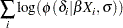
From a programming point of view, the second parameterization of the model is more difficult because the prior distribution on involves the data set variables seed and extract. Each prior distribution depends on a different set of observations in the input data set. Intuitively, you might think that the following statements would specify such a prior:
mu = beta0 + beta1*seed + beta2*extract + beta3*seed*extract;
prior delta ~ normal(mu, var = v);
However, this will not work. This is because the procedure is not able to match the observational level calculation (mu) with elements of a parameter array (there are 21 random effects in delta). Thus, the procedure cannot calculate the log of the prior density correctly. The solution is to cumulatively calculate the joint prior distribution for all  , and assign the prior distribution to all
  by using the GENERAL function.
The following statements generate Output 52.5.1:
proc mcmc data=seeds outpost=postout seed=332786 nmc=100000 thin=10
ntu=3000 monitor=(beta0-beta3 v);
ods select PostSummaries ess;
array delta[21];
parms delta: 0;
parms beta0 0 beta1 0 beta2 0 beta3 0 ;
parms v 1;
beginnodata;
sigma = sqrt(v);
endnodata;
w = beta0 + beta1*seed + beta2*extract + beta3*seed*extract;
if ind eq 1 then
lp = lpdfnorm(delta[ind], w, sigma);
else
lp = lp + lpdfnorm(delta[ind], w, sigma);
prior v ~ general(-log(v));
prior beta: ~ general(0);
prior delta: ~ general(lp);
pi = logistic(delta[ind]);
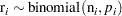
model r ~ binomial(n = n, p = pi);
run;
PROC MCMC statement specifies the input and output data sets, sets a seed for the random number generator, requests a very large simulation number, thins the Markov chain by 10, and specifies a tuning sample size of 3000. The MONITOR= option selects the parameters of interest. The ODS SELECT statement displays the summary statistics and effective sample size tables.
The ARRAY statement allocates an array of size 21 for the random effects parameter . There are three PARMS statements that place , and into three sampling blocks. Calculation of sigma does not involve any observations; hence, it is enclosed in the BEGINNODATA and ENDNODATA statements.
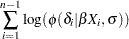
The next few lines of statements construct a joint prior distribution for all the parameters. The symbol w is the regression mean, whose value changes for every observation. The IF-ELSE statements add the log of the normal density to the symbol lp as PROC MCMC steps through the data set. When ind is 1, lp is the log of the normal density for delta[1] evaluated at the first regression mean w. As ind gradually increases to  , lp becomes
 |
which is the joint prior distribution for all .
The PRIOR statements assign three priors to these parameters, with noninformative priors on and . All of the delta parameters share a joint prior, which is defined by lp. Recall that PROC MCMC adds the log of the prior density to the log of the posterior density at the last observation at every simulation, so the expression lp will have the correct value.
Caution:You must define the expression lp before the PRIOR statement for the delta parameters. Switching the order of the PRIOR statement and the programming statements that define lp leads to an incorrect prior distribution for delta. The following statements are wrong because the expression lp has not completed its calculation when lp is added to the log of the posterior density at the last observation of the input data set.
prior delta: ~ general(lp);
w = beta0 + beta1*seed + beta2*extract + beta3*seed*extract;
if ind eq 1 then
   lp = lpdfnorm(delta[ind], w, sigma);
else
   lp = lp + lpdfnorm(delta[ind], w, sigma);
The prior you specify in this case is:
 |
The correct log density is the following:
 |
The symbol pi is the logit transformation. The MODEL specifies the response variable r as a binomial distribution with parameters n and pi.
The mixing is poor in this example. You can see from the effective sample size table (Output 52.5.1) that the efficiency for all parameters is relatively low, even after a substantial amount of thinning. One possible solution is to break the random effects block of parameters (b) into multiple blocks with a smaller number of parameters.
| Logistic Regression Random-Effects Model |
| Posterior Summaries | ||||||
|---|---|---|---|---|---|---|
| Parameter | N | Mean | Standard Deviation |
Percentiles | ||
| 25% | 50% | 75% | ||||
| beta0 | 10000 | -0.5503 | 0.2025 | -0.6784 | -0.5522 | -0.4193 |
| beta1 | 10000 | 0.0626 | 0.3292 | -0.1512 | 0.0653 | 0.2760 |
| beta2 | 10000 | 1.3546 | 0.2876 | 1.1732 | 1.3391 | 1.5349 |
| beta3 | 10000 | -0.8257 | 0.4498 | -1.1044 | -0.8255 | -0.5344 |
| v | 10000 | 0.1145 | 0.1019 | 0.0472 | 0.0875 | 0.1503 |
To fit the same model in PROC GLIMMIX, you can use the following statements, which produce Output 52.5.2:
proc glimmix data=seeds method=quad;
   ods select covparms parameterestimates;
   ods output covparms=cp parameterestimates=ps;
  class ind;
  model r/n = seed extract seed*extract/ dist=binomial link=logit solution;
  random intercept / subject=ind;
run;
It is hard to compare point estimates from these two procedures. However, you can visually compare the results by plotting a kernel density plot (by using the posterior sample from PROC MCMC output) on top of a normal approximation plot (by using the mean and standard error estimates from PROC GLIMMIX, for each parameter). This kernel comparison plot is shown in Output 52.5.3.
However, it takes some work to produce the kernel comparison plot. First, you must use PROC KDE to estimate the kernel density for each parameter from MCMC. Next, you want to get the point estimates from the PROC GLIMMIX output. Then, you generate a SAS data set that contains both the kernel density estimates and the gridded estimates based on normal approximations. Finally, you use PROC TEMPLATE (see Chapter 21, Statistical Graphics Using ODS ) to define an appropriate graphical template and produce the comparison plot by using PROC SGRENDER (see the SGRENDER Procedure in the SAS/GRAPH: Statistical Graphics Procedures Guide).
The following statements use PROC KDE on the posterior sample data set postout and estimate a kernel density for each parameter, saving the estimates to a SAS data set m1:
proc kde data=postout;
   univar beta0 beta1 beta2 beta3 v / out=m1 (drop=count);
run;
The following SAS statements take the estimates of all the parameters from the PROC GLIMMIX output, data sets ps and cp, and assign them to macro variables:
data gmxest(keep = parm mean sd);
   set ps cp;
   mean = estimate;
   sd = stderr;
   i = _n_-1;
   if(_n_ ne 5) then
      parm = "beta" || put(i, z1.);
   else
      parm = "var";
run;

data msd (keep=mean sd);
   set gmxest;
   do j = 1 to 401;
      output;
   end;
run;

data _null_;
   set ps;
   call symputx(compress(effect,'*'), estimate);
   call symputx(compress('s' || effect,'*'), stderr);
run;

data _null_;
   set cp;
   call symputx("var", estimate);
   call symputx("var_sd", stderr);
run;

%put &intercept &seed &extract &seedextract &var;
%put &sintercept &sseed &sextract &sseedextract &var_sd;
Specifically, the mean estimate of  is assigned to intercept, and the standard error of is assigned to sintercept. The macro variables seed, extract, seedextract are the mean estimates for
  ,
,  and
and  , respectively.
To create a SAS data set that contains both the kernel density estimates and the corresponding normal approximation, you can use the %REN and %RESHAPE macros. The %REN macro renames the variables of a SAS data set by appending the suffix name to each variable name, to avoid redundant variable names. The %RESHAPE macro takes an output data set from a PROC KDE run, and transposes it to the right format so that PROC SGRENDER can generate the right graph. The following statements define the %REN and %RESHAPE macros:
/* define macros */
%macro ren(in=, out=, suffix=);
   %local s;

   proc contents data=&in noprint out=__temp__(keep=name);
   run;

   data _null_;
      length s $ 32000;
      retain s;
      set __temp__ end=eof;
      s = trim(s)||' '||trim(name)||'='||compress(name||"&suffix");
      if eof then call symput('s', trim(s));
   run;

   proc datasets nolist;
      delete __temp__;
   run; quit;

   data &out;
      set &in(rename=(&s));
   run;
%mend;

%macro reshape(input, output, suffix1=, suffix2=);
   proc sort data=&input;
      by var;
   run;

   data tmp&input;
      set &input;
      by var;
      _n + 1;
      if first.var then _n = 0;
   run;

   proc sort;
      by _n var;
   run;

   proc transpose data=tmp&input out=_by_value_(drop=_n _name_ _label_);
      var value;
      by _n;
      id var;
   run;

   %ren(in=_by_value_, out=_by_value_, suffix=&suffix1)

   proc transpose data=tmp&input out=_by_den_(drop=_n _name_ _label_);
      var density;
      by _n;
      id var;
   run;

   %ren(in=_by_den_, out=_by_den_, suffix=&suffix2)

   data &output;
      merge _by_value_ _by_den_;
   run;

   proc datasets library=work;
      ods exclude all;
      delete tmp&input _by_value_ _by_den_;
   run;
   ods exclude none;
%mend;
When you apply the %RESHAPE macro to the data set m1, you create a SAS data set mcmc that has grid values of the parameters and their corresponding kernel density estimates. Next, you evaluate these parameter grid values in a normal density with the macro variables taken from the PROC GLIMMIX output:
/* create data set mcmc */
%reshape(m1, mcmc, suffix1=, suffix2=_kde);
data all;
   set mcmc;
   beta0_gmx = pdf('normal', beta0, &intercept, &sintercept);
   beta1_gmx = pdf('normal', beta1, &seed, &sseed);
   beta2_gmx = pdf('normal', beta2, &extract, &sextract);
   beta3_gmx = pdf('normal', beta3, &seedextract, &sseedextract);
   v_gmx = pdf('normal', v, &var, &var_sd);
run;
In the data set all, you have grid values on and , their kernel density estimates from PROC MCMC, and the normal density evaluated by using estimates from PROC GLIMMIX. To create an overlaid plot, you first use PROC TEMPLATE to create a  template as demonstrated by the following statements:
proc template;
   define statgraph twobythree;
      %macro plot;
         begingraph;
            layout lattice / rows=2 columns=3;
               %do i = 0 %to 3;
                  layout overlay /yaxisopts=(label=" ");
                     seriesplot y=beta&i._kde x=beta&i
                        / connectorder=xaxis
                          lineattrs=(pattern=mediumdash color=blue)
                        legendlabel = "MCMC Kernel" name="MCMC";
                     seriesplot y=beta&i._gmx x=beta&i
                        / connectorder=xaxis lineattrs=(color=red)
                        legendlabel="GLIMMIX Approximation" name="GLIMMIX";
                  endlayout;
               %end;
               layout overlay /yaxisopts=(label=" ")
                               xaxisopts=(linearopts=(viewmin=0 viewmax=0.6));
                  seriesplot y=v_kde x=v
                     / connectorder=xaxis
                       lineattrs=(pattern=mediumdash color=blue)
                     legendlabel = "MCMC Kernel" name="MCMC";
                  seriesplot y=v_gmx x=v
                     / connectorder=xaxis lineattrs=(color=red)
                     legendlabel="GLIMMIX Approximation" name="GLIMMIX";
               endlayout;
               Sidebar / align = bottom;
                  discretelegend "MCMC" "GLIMMIX";
               endsidebar;
            endlayout;
         endgraph;
      %mend; %plot;
   end;
run;
The kernel density comparison plot is produced by calling PROC SGRENDER (see the SGRENDER Procedure in the SAS/GRAPH: Statistical Graphics Procedures Guide):
proc sgrender data=all template=twobythree;
run;
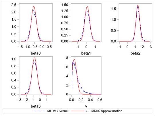
The kernel densities are very similar to each other. Kernel densities from PROC MCMC are not as smooth, possibly due to bad mixing of the Markov chains.
Nonlinear Poisson Regression Random-Effects Model
This example uses the pump failure data of Gaver and O’Muircheartaigh (1987). The number of failures and the time of operation are recorded for 10 pumps. Each of the pumps is classified into one of two groups corresponding to either continuous or intermittent operation. The following statements generate the data set:
title 'Nonlinear Poisson Regression Random Effects Model';
data pump;
   input y t group @@;
   pump = _n_;
   logtstd = log(t) - 2.4564900;
   datalines;
 5  94.320 1   1  15.720 2    5  62.880 1
14 125.760 1   3   5.240 2   19  31.440 1
 1   1.048 2   1   1.048 2    4   2.096 2
22  10.480 2
;
Each row denotes data for a single pump, and the variable logtstd contains the centered operation times. Letting  denote the number of failures for the
  th pump in the
  th group, Draper (1996) considers the following hierarchical model for these data:
 |
 |
 |
|||
 |
|
 |
|||
 |
|
 |
The model specifies different intercepts and slopes for each group, and the random effect is a mechanism for accounting for over-dispersion. You can use noninformative priors on the parameters  ,
,  , and .
 |
|
|
|||
|
|
|
The following statements fit this nonlinear hierarchical model and produce Output 52.5.4:
proc mcmc data=pump outpost=postout seed=248601 nmc=100000
          ntu=2000 thin=10
          monitor=(logsig beta1 beta2 alpha1 alpha2 s2 adif bdif);
   ods select PostSummaries;
   array alpha[2];
   array beta[2];
   array llambda[10];

   parms (alpha: beta:) 1;
   parms llambda: 1;
   parms s2 1;

   beginnodata;
   sd = sqrt(s2);
   logsig = log(s2)/2;
   adif = alpha1 - alpha2;
   bdif = beta1 - beta2;
   endnodata;
   w = alpha[group] + beta[group] * logtstd;
   if pump eq 1 then
      lp = lpdfnorm(llambda[pump], w, sd);
   else
      lp = lp + lpdfnorm(llambda[pump], w, sd);
   prior alpha: beta: ~ general(0);
   prior s2 ~ general(-log(s2));
   prior llambda: ~ general(lp);

   lambda = exp(llambda[pump]);
   model y ~ poisson(lambda);
run;
The PROC MCMC statement specifies the input data set (pump), the output data set (postout), a seed for the random number generator, and an MCMC sample of 100000. It also requests a tuning sample size of 2000 and a thinning rate of 10. The MONITOR= option keeps track of a number of parameters and symbols in the model. The five parameters are beta1, beta2, alpha1, alpha2, and s2. The symbol logsig is the log of the standard deviation, adif measures the difference between alpha1 and alpha2, and bdif measures the difference between beta1 and beta2. The ODS SELECT statement displays the summary statistics table.
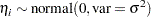
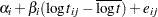
Modeling the random effects  with a normal distribution with mean 0 and variance is equivalent to modeling
  with a normal distribution with mean
 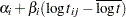 and variance . Here again, the prior distribution on depends on the data set variable logstd; hence, the construction of the prior must take place before the PRIOR statement for . The symbol lp keeps track of the cumulative log prior density for .
The symbol lambda is the exponential of the corresponding , and the MODEL statement gives the response variable y a Poisson likelihood with a mean parameter lambda.
The posterior summary statistics table is shown in Output 52.5.4.
| Nonlinear Poisson Regression Random Effects Model |
| Posterior Summaries | ||||||
|---|---|---|---|---|---|---|
| Parameter | N | Mean | Standard Deviation |
Percentiles | ||
| 25% | 50% | 75% | ||||
| logsig | 10000 | 0.1045 | 0.3862 | -0.1563 | 0.0883 | 0.3496 |
| beta1 | 10000 | -0.4467 | 1.2818 | -1.1641 | -0.4421 | 0.2832 |
| beta2 | 10000 | 0.5858 | 0.5808 | 0.2376 | 0.5796 | 0.9385 |
| alpha1 | 10000 | 2.9719 | 2.3658 | 1.6225 | 2.9612 | 4.3137 |
| alpha2 | 10000 | 1.6406 | 0.8674 | 1.1429 | 1.6782 | 2.1673 |
| s2 | 10000 | 1.7004 | 1.7995 | 0.7316 | 1.1931 | 2.0121 |
| adif | 10000 | 1.3313 | 2.4934 | -0.1670 | 1.2669 | 2.8032 |
| bdif | 10000 | -1.0325 | 1.4186 | -1.8379 | -1.0284 | -0.2189 |
Draper (1996) reports a posterior mean and standard deviation as follows:  ,
,  ,
,  , and
, and  . Most estimates from Output 52.5.4 agree with Draper’s estimates, with the exception of
  . The difference might be attributed to the different set of prior distributions on , , and
  that are used in this analysis.
You can also use PROC NLMIXED to fit the same model. The following statements run PROC NLMIXED and produce Output 52.5.5:
proc nlmixed data=pump;
   ods select parameterestimates additionalestimates;
   ods output additionalestimates=cp parameterestimates=ps;
   parms logsig 0 beta1 1 beta2 1 alpha1 1 alpha2 1;
   if (group = 1) then eta = alpha1 + beta1*logtstd + e;
   else eta = alpha2 + beta2*logtstd + e;
   lambda = exp(eta);
   model y ~ poisson(lambda);
   random e ~ normal(0,exp(2*logsig)) subject=pump;
   estimate 'adif' alpha1-alpha2;
   estimate 'bdif' beta1-beta2;
   estimate 's2' exp(2*logsig);
run;
| Nonlinear Poisson Regression Random Effects Model |
| Parameter Estimates | |||||||||
|---|---|---|---|---|---|---|---|---|---|
| Parameter | Estimate | Standard Error | DF | t Value | Pr > |t| | Alpha | Lower | Upper | Gradient |
| logsig | -0.3161 | 0.3213 | 9 | -0.98 | 0.3508 | 0.05 | -1.0429 | 0.4107 | -0.00002 |
| beta1 | -0.4256 | 0.7473 | 9 | -0.57 | 0.5829 | 0.05 | -2.1162 | 1.2649 | -0.00002 |
| beta2 | 0.6097 | 0.3814 | 9 | 1.60 | 0.1443 | 0.05 | -0.2530 | 1.4724 | -1.61E-6 |
| alpha1 | 2.9644 | 1.3826 | 9 | 2.14 | 0.0606 | 0.05 | -0.1632 | 6.0921 | -5.25E-6 |
| alpha2 | 1.7992 | 0.5492 | 9 | 3.28 | 0.0096 | 0.05 | 0.5568 | 3.0415 | -5.73E-6 |
Again, the point estimates from PROC NLMIXED for the mean parameters agree relatively closely with the Bayesian posterior means. You can note that there are differences in the likelihood-based standard errors. This is most likely due to the fact that the Bayesian standard deviations account for the uncertainty in estimating , whereas the likelihood approach plugs in its estimated value.
You can do a similar kernel density plot that compares the PROC MCMC results, the PROC NLMIXED results and those reported by Draper. The following statements generate Output 52.5.6:
data nlmest(keep = parm mean sd);
   set ps cp;
   mean = estimate;
   sd = standarderror;
   if _n_ <= 5 then
      parm = parameter;
   else
      parm = label;
run;

data msd (keep=mean sd);
   set nlmest;
   do j = 1 to 401;
      output;
   end;
run;

data _null_;
   set ps;
   call symputx(compress('m' || parameter,'*'), estimate);
   call symputx(compress('s' || parameter,'*'), standarderror);
run;

data _null_;
   set cp;
   call symputx(compress('m' || label,'*'), estimate);
   call symputx(compress('s' || label,'*'), standarderror);
run;

%put &mlogsig &mbeta1 &mbeta2 &malpha1 &malpha2 &madif &mbdif &ms2;
%put &slogsig &sbeta1 &sbeta2 &salpha1 &salpha2 &sadif &sbdif &ss2;

proc kde data=postout;
   univar logsig beta1 beta2 alpha1 alpha2 adif bdif s2 / out=m1 (drop=count);
run;

%reshape(m1, mcmc, suffix1=, suffix2=_kde);

data all;
   set mcmc;
   logsig_nlm = pdf('normal', logsig, &mlogsig, &slogsig);
   alpha1_nlm = pdf('normal', alpha1, &malpha1, &salpha1);
   alpha2_nlm = pdf('normal', alpha2, &malpha2, &salpha2);
   beta1_nlm = pdf('normal', beta1, &mbeta1, &sbeta1);
   beta2_nlm = pdf('normal', beta2, &mbeta2, &sbeta2);
   adif_nlm = pdf('normal', adif, &madif, &sadif);
   bdif_nlm = pdf('normal', bdif, &mbdif, &sbdif);
   s2_nlm = pdf('normal', s2, &ms2, &ss2);
   logsig_draper = pdf('normal', logsig, 0.28, 0.42);
   beta1_draper = pdf('normal', beta1, -0.45, 1.5);
   beta2_draper = pdf('normal', beta2, 0.63, 0.68);
   adif_draper = pdf('normal', adif, 1.3, 3.0);
run;

proc template;
   define statgraph threebythree;
      %macro plot;
         begingraph;
            layout lattice / rows=3 columns=3;
               layout overlay /yaxisopts=(label=" ");
                  seriesplot y=logsig_kde x=logsig
                     / connectorder=xaxis
                       lineattrs=(pattern=mediumdash color=blue)
                     legendlabel = "MCMC Kernel" name="MCMC";
                  seriesplot y=logsig_nlm x=logsig
                     / connectorder=xaxis lineattrs=(color=red)
                     legendlabel = "NLMIXED Approximation" name="NLMIXED";
                  seriesplot y=logsig_draper x=logsig
                     / connectorder=xaxis
                       lineattrs=(pattern=shortdash color=green)
                     legendlabel = "Draper (1996) Approximation" name="Draper";
               endlayout;
               %do i = 1 %to 2;
                  layout overlay /yaxisopts=(label=" ");
                     seriesplot y=alpha&i._kde x=alpha&i
                        / connectorder=xaxis
                          lineattrs=(pattern=mediumdash color=blue)
                        legendlabel = "MCMC Kernel" name="MCMC";
                     seriesplot y=alpha&i._nlm x=alpha&i
                        / connectorder=xaxis lineattrs=(color=red)
                        legendlabel = "NLMIXED Approximation" name="NLMIXED";
                  endlayout;
               %end;
               %do i = 1 %to 2;
                  layout overlay /yaxisopts=(label=" ");
                     seriesplot y=beta&i._kde x=beta&i
                        / connectorder=xaxis
                          lineattrs=(pattern=mediumdash color=blue)
                        legendlabel = "MCMC Kernel" name="MCMC";
                     seriesplot y=beta&i._nlm x=beta&i
                        / connectorder=xaxis lineattrs=(color=red)
                        legendlabel = "NLMIXED Approximation" name="NLMIXED";
                     seriesplot y=beta&i._draper x=beta&i
                        / connectorder=xaxis
                          lineattrs=(pattern=shortdash color=green)
                        legendlabel = "Draper (1996) Approximation" name="Draper";
                  endlayout;
               %end;
               layout overlay /yaxisopts=(label=" ");
                  seriesplot y=adif_kde x=adif
                     / connectorder=xaxis
                       lineattrs=(pattern=mediumdash color=blue)
                     legendlabel = "MCMC Kernel" name="MCMC";
                  seriesplot y=adif_nlm x=adif
                     / connectorder=xaxis lineattrs=(color=red)
                     legendlabel = "NLMIXED Approximation" name="NLMIXED";
                  seriesplot y=adif_draper x=adif
                     / connectorder=xaxis
                       lineattrs=(pattern=shortdash color=green)
                     legendlabel = "Draper (1996) Approximation" name="Draper";
               endlayout;
               layout overlay /yaxisopts=(label=" ");
                  seriesplot y=bdif_kde x=bdif
                     / connectorder=xaxis
                       lineattrs=(pattern=mediumdash color=blue)
                     legendlabel = "MCMC Kernel" name="MCMC";
                  seriesplot y=bdif_nlm x=bdif
                     / connectorder=xaxis lineattrs=(color=red)
                     legendlabel = "NLMIXED Approximation" name="NLMIXED";
               endlayout;
               layout overlay /yaxisopts=(label=" ")
                               xaxisopts=(linearopts=(viewmin=0 viewmax=5));
                  seriesplot y=s2_kde x=s2
                     / connectorder=xaxis
                       lineattrs=(pattern=mediumdash color=blue)
                     legendlabel = "MCMC Kernel" name="MCMC";
                  seriesplot y=s2_nlm x=s2
                     / connectorder=xaxis lineattrs=(color=red)
                     legendlabel = "NLMIXED Approximation" name="NLMIXED";
               endlayout;
               Sidebar / align = bottom;
                  discretelegend "MCMC" "NLMIXED" "Draper";
               endsidebar;
            endlayout;
         endgraph;
      %mend; %plot;
   end;
run;

proc sgrender data=all template=threebythree;
run;
The macro %RESHAPE is defined in the example Logistic Regression Random-Effects Model.
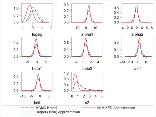
Copyright © SAS Institute, Inc. All Rights Reserved.