This example illustrates how you can fit a mixed-effects model in PROC MCMC. PROC MCMC offers you the ability to model beyond the normal likelihood (see Random-Effects Models), and you can model as many levels of random effects as are needed with this procedure.

Consider a scenario in which data are collected in groups and you wish to model group-specific effects. You can use a mixed-effects model (sometimes also known as a random-effects model or a variance-components model):

where is the group index and indexes the observations in the th group. In the regression model, the fixed effects and are the intercept and the coefficient for variable , respectively. The random effects is the mean for the th group, and are the error term.

Consider the following SAS data set:

title 'Mixed-Effects Model';
 
data heights;
   input Family G$ Height @@;
   datalines;
1 F 67   1 F 66   1 F 64   1 M 71   1 M 72   2 F 63
2 F 63   2 F 67   2 M 69   2 M 68   2 M 70   3 F 63
3 M 64   4 F 67   4 F 66   4 M 67   4 M 67   4 M 69
;
 
data input;
   set heights;
   if g eq 'F' then gender = 1;
   else gender = 0;
   drop g;
run;

The response variable Height measures the heights (in inches) of 18 individuals. The individuals are classified according to Family and Gender.

Height is assumed to be normally distributed:

which corresponds to a normal likelihood as follows:

The priors on the parameters , , are assumed to be normal as well:

Priors on the variance terms, and , are inverse-gamma:

where denotes the density function of an inverse-gamma distribution.

The following statements fit a linear random-effects model to the data and produce the output shown in Figure 52.9 and Figure 52.10:

ods graphics on;
proc mcmc data=input outpost=postout thin=10 nmc=50000 seed=7893
          monitor=(b0 b1);
   ods select PostSummaries PostIntervals tadpanel;
   array gamma[4];
 
   parms b0 0 b1 0 gamma: 0;
   parms s2 1 ;
   parms s2g 1;
 
   prior b: ~ normal(0, var = 10000);
   prior gamma: ~ normal(0, var = s2g);
   prior s2: ~ igamma(0.001, scale = 1000);
 
   mu = b0 + b1 * gender + gamma[family];
   model height ~ normal(mu, var = s2);
run;
ods graphics off;

The statements are very similar to those shown in the previous two examples. The ODS GRAPHICS ON statement requests ODS Graphics. The PROC MCMC statement specifies the input and output data sets, the simulation size, the thinning rate, and a random number seed. The MONITOR= option indicates that the model parameters b0 and b1 are the quantities of interest. The ODS SELECT statement displays the summary statistics table, the interval statistics table, and the diagnostics plots.

The ARRAY statement defines a one-dimensional array, gamma, with 4 elements. You can refer to the array elements with variable names (gamma1 to gamma4 by default) or with subscripts, such as gamma[2]. To indicate subscripts, you must use either brackets or braces , but not parentheses . Note that this is different from the way subscripts are indicated in the DATA step. See the section ARRAY Statement for more information.

The PRIOR statements specify priors for all the parameters. The notation b: is a shorthand for all symbols that start with the letter ‘b’. In this example, it includes b0 and b1. Similarly, gamma: stands for all four gamma parameters, and s2: stands for both s2 and s2g. This shorthand notation can save you some typing, and it keeps your statements tidy.

The mu assignment statement calculates the expected value of height in the random-effects model. The symbol family is a data set variable that indexes family. Here gamma[family] is the random effect for the value of family.

Finally, the MODEL statement specifies the likelihood function for height.

The posterior summary and interval statistics for b0 and b1 are shown in Figure 52.9.

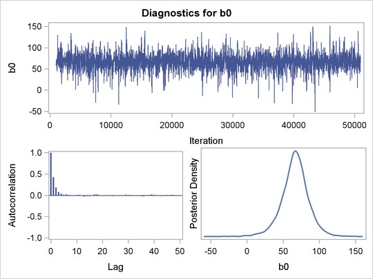
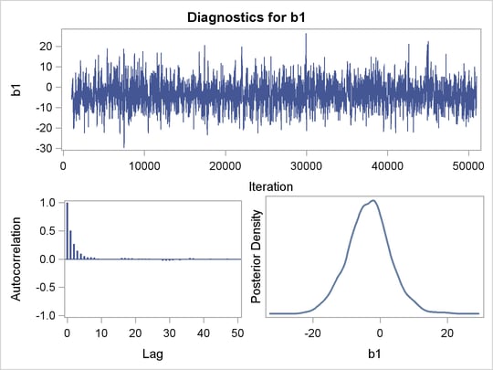
Trace plots, autocorrelation plots, and posterior density plots for b1 and logpost are shown in Figure 52.10. The mixing of b1 looks good. The convergence plots for the other parameters also look reasonable, and are not shown here.

Figure 52.10 Plots for and Log of the Posterior Density

From the interval statistics table, you see that both the equal-tail and HPD intervals for are positive, strongly indicating the positive effect of the parameter. On the other hand, both intervals for cover the value zero, indicating that gender does not have a strong impact on predicting height in this model.