| The MCMC Procedure |
Example 52.3 Generalized Linear Models
This example discusses two examples of fitting generalized linear models (GLM) with PROC MCMC. One uses a logistic regression model and one uses a Poisson regression model. The logistic examples use both a diffuse prior and a Jeffreys’ prior on the regression coefficients. You can also use the BAYES statement in PROC GENMOD. See Chapter 37, The GENMOD Procedure.
Logistic Regression Model with a Diffuse Prior
The following statements create a SAS data set with measurements of the number of deaths, y, among n beetles that have been exposed to an environmental contaminant x:
title 'Logistic Regression Model with a Diffuse Prior';
data beetles;
   input n y x @@;
   datalines;
6  0  25.7   8  2  35.9   5  2  32.9   7  7  50.4   6  0  28.3
7  2  32.3   5  1  33.2   8  3  40.9   6  0  36.5   6  1  36.5
6  6  49.6   6  3  39.8   6  4  43.6   6  1  34.1   7  1  37.4
8  2  35.2   6  6  51.3   5  3  42.5   7  0  31.3   3  2  40.6
;
You can model the data points  with a binomial distribution:
 |
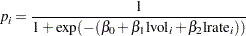
where  is the success probability and links to the regression covariate
  through a logit transformation:
 |
The priors on  and
and  are both diffuse normal:
 |
 |
 |
|||
 |
|
|
These statements fit a logistic regression with PROC MCMC:
ods graphics on;
proc mcmc data=beetles ntu=1000 nmc=20000 nthin=2 propcov=quanew
          diag=(mcse ess) outpost=beetleout seed=246810;
   ods select PostSummaries PostIntervals mcse ess TADpanel;
   parms (alpha  beta) 0;
   prior alpha beta ~ normal(0, var = 10000);
   p = logistic(alpha + beta*x);
   model y ~ binomial(n,p);
run;
The key statement in the program is the assignment to p that calculates the probability of death. The SAS function LOGISTIC does the proper transformation. The MODEL statement specifies that the response variable, y, is binomially distributed with parameters n (from the input data set) and p. The summary statistics table, interval statistics table, the Monte Carlos standard error table, and the effective sample sizes table are shown in Output 52.3.1.
| Logistic Regression Model with a Diffuse Prior |
| Posterior Summaries | ||||||
|---|---|---|---|---|---|---|
| Parameter | N | Mean | Standard Deviation |
Percentiles | ||
| 25% | 50% | 75% | ||||
| alpha | 10000 | -11.7707 | 2.0997 | -13.1243 | -11.6683 | -10.3003 |
| beta | 10000 | 0.2920 | 0.0542 | 0.2537 | 0.2889 | 0.3268 |
| Posterior Intervals | |||||
|---|---|---|---|---|---|
| Parameter | Alpha | Equal-Tail Interval | HPD Interval | ||
| alpha | 0.050 | -16.3332 | -7.9675 | -15.8822 | -7.6673 |
| beta | 0.050 | 0.1951 | 0.4087 | 0.1901 | 0.4027 |
The summary statistics table shows that the sample mean of the output chain for the parameter alpha is  . This is an estimate of the mean of the marginal posterior distribution for the intercept parameter alpha. The estimated posterior standard deviation for alpha is 2.0997. The two
  credible intervals for alpha are both negative, which indicates with very high probability that the intercept term is negative. On the other hand, you observe a positive effect on the regression coefficient beta. Exposure to the environment contaminant increases the probability of death.
The Monte Carlo standard errors of each parameter are significantly small relative to the posterior standard deviations. A small MCSE/SD ratio indicates that the Markov chain has stabilized and the mean estimates do not vary much over time. Note that the precision in the parameter estimates increases with the square of the MCMC sample size, so if you want to double the precision, you must quadruple the MCMC sample size.
MCMC chains do not produce independent samples. Each sample point depends on the point before it. In this case, the correlation time estimate, read from the effective sample sizes table, is roughly 4. This means that it takes four observations from the MCMC output to make inferences about alpha with the same precision that you would get from using an independent sample. The effective sample size of 2470 reflects this loss of efficiency. The coefficient beta has similar efficiency. You can often observe that some parameters have significantly better mixing (better efficiency) than others, even in a single Markov chain run.
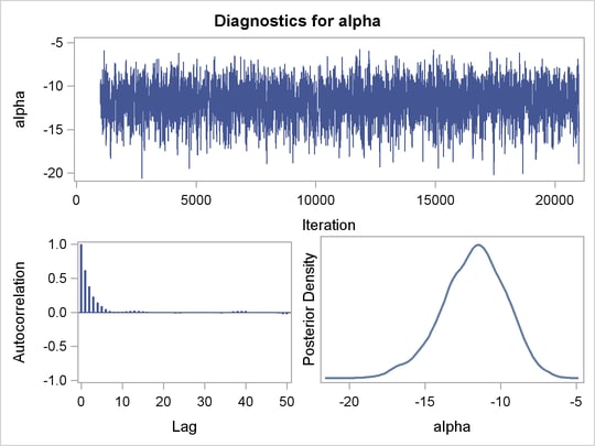
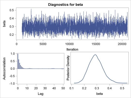
Trace plots and autocorrelation plots of the posterior samples are shown in Output 52.3.2. Convergence looks good in both parameters; there is good mixing in the trace plot and quick drop-off in the ACF plot.
One advantage of Bayesian methods is the ability to directly answer scientific questions. In this example, you might want to find out the posterior probability that the environmental contaminant increases the probability of death—that is,  . This can be estimated using the following steps:
proc format;
   value betafmt low-0 = 'beta <= 0' 0<-high = 'beta > 0';
run;

proc freq data=beetleout;
   tables beta /nocum;
   format beta betafmt.;
run;
All of the simulated values for are greater than zero, so the sample estimate of the posterior probability that  is 100%. The evidence overwhelmingly supports the hypothesis that increased levels of the environmental contaminant increase the probability of death.
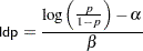
If you are interested in making inference based on any quantities that are transformations of the random variables, you can either do it directly in PROC MCMC or by using the DATA step after you run the simulation. Transformations sometimes can make parameter inference quite formidable using direct analytical methods, but with simulated chains, it is easy to compute chains for any set of parameters. Suppose that you are interested in the lethal dose and want to estimate the level of the covariate x that corresponds to a probability of death,  . Abbreviate this quantity as ldp. In other words, you want to solve the logit transformation with a fixed value . The lethal dose is as follows:
 |
You can obtain an estimate of any ldp by using the posterior mean estimates for and . For example, lp95, which corresponds to  , is calculated as follows:
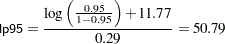 |
where  and
and  are the posterior mean estimates of and , respectively, and
  is the estimated lethal dose that leads to a death rate.
While it is easy to obtain the point estimates, it is harder to estimate other posterior quantities, such as the standard deviation directly. However, with PROC MCMC, you can trivially get estimates of any posterior quantities of lp95. Consider the following program in PROC MCMC:
proc mcmc data=beetles ntu=1000 nmc=20000 nthin=2 propcov=quanew
          outpost=beetleout seed=246810 plot=density
          monitor=(pi30 ld05 ld50 ld95);
   ods select PostSummaries PostIntervals densitypanel;
   parms (alpha  beta) 0;
   begincnst;
      c1 = log(0.05 / 0.95);
      c2 = -c1;
   endcnst;

   beginnodata;
   prior alpha beta ~ normal(0, var = 10000);
   pi30 = logistic(alpha + beta*30);
   ld05 = (c1 - alpha) / beta;
   ld50 = - alpha / beta;
   ld95 = (c2 - alpha) / beta;
   endnodata;
   pi = logistic(alpha + beta*x);
   model y ~ binomial(n,pi);
run;
ods graphics off;
The program estimates four additional posterior quantities. The three lpd quantities, ld05, ld50, and ld95, are the three levels of the covariate that kills 5%, 50%, and 95% of the population, respectively. The predicted probability when the covariate x takes the value of 30 is pi30. The MONITOR= option selects the quantities of interest. The PLOTS= option selects kernel density plots as the only ODS graphical output, excluding the trace plot and autocorrelation plot.
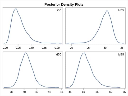
Programming statements between the BEGINCNST and ENDCNST statements define two constants. These statements are executed once at the beginning of the simulation. The programming statements between the BEGINNODATA and ENDNODATA statements evaluate the quantities of interest. The symbols, pi30, ld05, ld50, and ld95, are functions of the parameters alpha and beta only. Hence, they should not be processed at the observation level and should be included in the BEGINNODATA and ENDNODATA statements. Output 52.3.4 lists the posterior summary and Output 52.3.5 shows the density plots of these posterior quantities.
| Logistic Regression Model with a Diffuse Prior |
| Posterior Summaries | ||||||
|---|---|---|---|---|---|---|
| Parameter | N | Mean | Standard Deviation |
Percentiles | ||
| 25% | 50% | 75% | ||||
| pi30 | 10000 | 0.0524 | 0.0253 | 0.0340 | 0.0477 | 0.0662 |
| ld05 | 10000 | 29.9281 | 1.8814 | 28.8430 | 30.1727 | 31.2563 |
| ld50 | 10000 | 40.3745 | 0.9377 | 39.7271 | 40.3165 | 40.9612 |
| ld95 | 10000 | 50.8210 | 2.5353 | 49.0372 | 50.5157 | 52.3100 |
The posterior mean estimate of lp95 is  , which is close to the estimate of by using the posterior mean estimates of the parameters. With PROC MCMC, in addition to the mean estimate, you can get the standard deviation, quantiles, and interval estimates at any level of significance.
From the density plots, you can see, for example, that the sample distribution for  is skewed to the right, and almost all of your posterior belief concerning is concentrated in the region between zero and 0.15.
It is easy to use the DATA step to calculate these quantities of interest. The following DATA step uses the simulated values of and to create simulated values from the posterior distributions of ld05, ld50, ld95, and :
data transout;
   set beetleout;
   pi30 = logistic(alpha + beta*30);
   ld05 = (log(0.05 / 0.95) - alpha) / beta;
   ld50 = (log(0.50 / 0.50) - alpha) / beta;
   ld95 = (log(0.95 / 0.05) - alpha) / beta;
run;
Subsequently, you can use SAS/INSIGHT, or the UNIVARIATE, CAPABILITY, or KDE procedures to analyze the posterior sample. If you want to regenerate the default ODS graphs from PROC MCMC, see Regenerating Diagnostics Plots.
Logistic Regression Model with Jeffreys’ Prior
A controlled experiment was run to study the effect of the rate and volume of air inspired on a transient reflex vasoconstriction in the skin of the fingers. Thirty-nine tests under various combinations of rate and volume of air inspired were obtained (Finney; 1947). The result of each test is whether or not vasoconstriction occurred. Pregibon (1981) uses this set of data to illustrate the diagnostic measures he proposes for detecting influential observations and to quantify their effects on various aspects of the maximum likelihood fit. The following statements create the data set vaso:
title 'Logistic Regression Model with Jeffreys Prior';
data vaso;
   input vol rate resp @@;
   lvol = log(vol);
   lrate = log(rate);
   ind = _n_;
   cnst = 1;
   datalines;
3.7  0.825  1  3.5  1.09  1  1.25  2.5   1  0.75  1.5  1
0.8  3.2    1  0.7  3.5   1  0.6   0.75  0  1.1   1.7  0
0.9  0.75   0  0.9  0.45  0  0.8   0.57  0  0.55  2.75 0
0.6  3.0    0  1.4  2.33  1  0.75  3.75  1  2.3  1.64  1
3.2  1.6    1  0.85 1.415 1  1.7   1.06  0  1.8  1.8   1
0.4  2.0    0  0.95 1.36  0  1.35  1.35  0  1.5  1.36  0
1.6  1.78   1  0.6  1.5   0  1.8   1.5   1  0.95 1.9   0
1.9  0.95   1  1.6  0.4   0  2.7   0.75  1  2.35 0.03  0
1.1  1.83   0  1.1  2.2   1  1.2   2.0   1  0.8  3.33  1
0.95 1.9    0  0.75 1.9   0  1.3   1.625 1
;
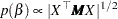
The variable resp represents the outcome of a test. The variable lvol represents the log of the volume of air intake, and the variable lrate represents the log of the rate of air intake. You can model the data by using logistic regression. You can model the response with a binary likelihood:
 |
with
 |
Let  be the design matrix in the regression. Jeffreys’ prior for this model is
 |
where  is a
is a  by matrix with off-diagonal elements being
  and diagonal elements being
  . For details on Jeffreys’ prior, see Jeffreys’ Prior. You can use a number of matrix functions, such as the determinant function, in PROC MCMC to construct Jeffreys’ prior. The following statements illustrate how to fit a logistic regression with Jeffreys’ prior:
/* fitting a logistic regression with Jeffreys' prior */
%let n = 39;
proc mcmc data=vaso nmc=10000 outpost=mcmcout seed=17;
   ods select PostSummaries PostIntervals;

   array beta[3] beta0 beta1 beta2;
   array m[&n, &n];
   array x[&n, 3];
   array xt[3, &n];
   array xtm[3, &n];
   array xmx[3, 3];
   array p[&n];

   parms beta0 1 beta1 1 beta2 1;

   begincnst;
      x[ind, 1] = 1;
      x[ind, 2] = lvol;
      x[ind, 3] = lrate;
      if (ind eq &n) then do;
         call transpose(x, xt);
         call zeromatrix(m);
      end;
   endcnst;

   beginnodata;
   call mult(x, beta, p);              /* p = x * beta */
   do i = 1 to &n;
      p[i] = 1 / (1 + exp(-p[i]));     /* p[i] = 1/(1+exp(-x*beta)) */
      m[i,i] = p[i] * (1-p[i]);
   end;
   call mult (xt, m, xtm);             /* xtm = xt * m        */
   call mult (xtm, x, xmx);            /* xmx = xtm * x       */
   call det (xmx, lp);                 /* lp = det(xmx)       */
   lp = 0.5 * log(lp);                 /* lp = -0.5 * log(lp) */
   prior beta: ~ general(lp);
   endnodata;

   model resp ~ bern(p[ind]);
run;
The first ARRAY statement defines an array beta with three elements: beta0, beta1, and beta2. The subsequent statements define arrays that are used in the construction of Jeffreys’ prior. These include m (the matrix), x (the design matrix), xt (the transpose of x), and some additional work spaces.
The explanatory variables lvol and lrate are saved in the array x in the BEGINCNST and ENDCNST statements. See BEGINCNST/ENDCNST Statement for details. After all the variables are read into x, you transpose the x matrix and store it to xt. The ZEROMATRIX function call assigns all elements in matrix m the value zero. To avoid redundant calculation, it is best to perform these calculations as the last observation of the data set is processed—that is, when ind is 39.
You calculate Jeffreys’ prior in the BEGINNODATA and ENDNODATA statements. The probability vector p is the product of the design matrix x and parameter vector beta. The diagonal elements in the matrix m are . The expression lp is the logarithm of Jeffreys’ prior. The PRIOR statement assigns lp as the prior for the regression coefficients. The MODEL statement assigns a binary likelihood to resp, with probability p[ind]. The p array is calculated earlier using the matrix function MULT. You use the ind variable to pick out the right probability value for each resp.
Posterior summary statistics are displayed in Output 52.3.6.
You can also use PROC GENMOD to fit the same model by using the following statements:
proc genmod data=vaso descending;
   ods select PostSummaries PostIntervals;
   model resp = lvol lrate / d=bin link=logit;
   bayes seed=17 coeffprior=jeffreys nmc=20000 thin=2;
run;
The MODEL statement indicates that resp is the response variable and lvol and lrate are the covariates. The options in the MODEL statement specify a binary likelihood and a logit link function. The BAYES statement requests Bayesian capability. The SEED=, NMC=, and THIN= arguments work in the same way as in PROC MCMC. The COEFFPRIOR=JEFFREYS option requests Jeffreys’ prior in this analysis.
The PROC GENMOD statements produce Output 52.3.7, with estimates very similar to those reported in Output 52.3.6. Note that you should not expect to see identical output from PROC GENMOD and PROC MCMC, even with the simulation setup and identical random number seed. The two procedures use different sampling algorithms. PROC GENMOD uses the adaptive rejection metropolis algorithm (ARMS) (Gilks and Wild; 1992; Gilks; 2003) while PROC MCMC uses a random walk Metropolis algorithm. The asymptotic answers, which means that you let both procedures run an very long time, would be the same as they both generate samples from the same posterior distribution.
| Logistic Regression Model with Jeffreys Prior |
| Posterior Summaries | ||||||
|---|---|---|---|---|---|---|
| Parameter | N | Mean | Standard Deviation |
Percentiles | ||
| 25% | 50% | 75% | ||||
| Intercept | 10000 | -2.8731 | 1.3088 | -3.6754 | -2.7248 | -1.9253 |
| lvol | 10000 | 5.1639 | 1.8087 | 3.8451 | 4.9475 | 6.2613 |
| lrate | 10000 | 4.5501 | 1.8071 | 3.2250 | 4.3564 | 5.6810 |
Poisson Regression
You can use the Poisson distribution to model the distribution of cell counts in a multiway contingency table. Aitkin et al. (1989) have used this method to model insurance claims data. Suppose the following hypothetical insurance claims data are classified by two factors: age group (with two levels) and car type (with three levels). The following statements create the data set:
title 'Poisson Regression';
data insure;
   input n c car $ age;
   ln = log(n);
   if car = 'large' then
      do car_dummy1=1;
         car_dummy2=0;
      end;
   else if car = 'medium' then
      do car_dummy1=0;
         car_dummy2=1;
      end;
   else
      do car_dummy1=0;
         car_dummy2=0;
      end;

   datalines;
   500   42  small  0
   1200  37  medium 0
   100    1  large  0
   400  101  small  1
   500   73  medium 1
   300   14  large  1
   ;
The variable n represents the number of insurance policy holders and the variable c represents the number of insurance claims. The variable car is the type of car involved (classified into three groups), and it is coded into two levels. The variable age is the age group of a policy holder (classified into two groups).
Assume that the number of claims c has a Poisson probability distribution and that its mean,  , is related to the factors car and age for observation
  by
by
 |
 |
 |
|||
 |
|
 |
|||
|
|
 |
|||
|
|
 |
The indicator variables  is associated with the
  th level of the variable car for observation in the following way:
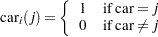 |
A similar coding applies to age. The ’s are parameters. The logarithm of the variable n is used as an offset—that is, a regression variable with a constant coefficient of 1 for each observation. Having the offset constant in the model is equivalent to fitting an expanded data set with 3000 observations, each with response variable y observed on an individual level. The log link is used to relate the mean and the factors car and age.
The following statements run PROC MCMC:
proc mcmc data=insure outpost=insureout nmc=5000 propcov=quanew
          maxtune=0 seed=7;
   ods select PostSummaries PostIntervals;
   parms alpha 0 beta_car1 0 beta_car2 0 beta_age 0;
   prior alpha beta: ~ normal(0, prec = 1e-6);

   mu = ln + alpha + beta_car1 * car_dummy1
      + beta_car2 * car_dummy2 + beta_age * age;
   model c ~ poisson(exp(mu));
run;
The analysis uses a relatively flat prior on all the regression coefficients, with mean at and precision at  . The option MAXTUNE=0 skips the tuning phase because the optimization routine (PROPCOV=QUANEW) provides good initial values and proposal covariance matrix.
There are four parameters in the model: alpha is the intercept; beta_car1 and beta_car2 are coefficients for the class variable car, which has three levels; and beta_age is the coefficient for age. The symbol mu connects the regression model and the Poisson mean by using the log link. The MODEL statement specifies a Poisson likelihood for the response variable c.
Posterior summary and interval statistics are shown in Output 52.3.8.
| Poisson Regression |
| Posterior Summaries | ||||||
|---|---|---|---|---|---|---|
| Parameter | N | Mean | Standard Deviation |
Percentiles | ||
| 25% | 50% | 75% | ||||
| alpha | 5000 | -2.6403 | 0.1344 | -2.7261 | -2.6387 | -2.5531 |
| beta_car1 | 5000 | -1.8335 | 0.2917 | -2.0243 | -1.8179 | -1.6302 |
| beta_car2 | 5000 | -0.6931 | 0.1255 | -0.7775 | -0.6867 | -0.6118 |
| beta_age | 5000 | 1.3151 | 0.1386 | 1.2153 | 1.3146 | 1.4094 |
To fit the same model by using PROC GENMOD, you can do the following. Note that the default normal prior on the coefficients is  , the same as used in the PROC MCMC. The following statements run PROC GENMOD and create Output 52.3.9:
proc genmod data=insure;
   ods select PostSummaries PostIntervals;
   class car age(descending);
   model c = car age / dist=poisson link=log offset=ln;
   bayes seed=17 nmc=5000 coeffprior=normal;
run;
To compare, posterior summary and interval statistics from PROC GENMOD are reported in Output 52.3.9, and they are very similar to PROC MCMC results in Output 52.3.8.
| Poisson Regression |
| Posterior Summaries | ||||||
|---|---|---|---|---|---|---|
| Parameter | N | Mean | Standard Deviation |
Percentiles | ||
| 25% | 50% | 75% | ||||
| Intercept | 5000 | -2.6353 | 0.1299 | -2.7243 | -2.6312 | -2.5455 |
| carlarge | 5000 | -1.7996 | 0.2752 | -1.9824 | -1.7865 | -1.6139 |
| carmedium | 5000 | -0.6977 | 0.1269 | -0.7845 | -0.6970 | -0.6141 |
| age1 | 5000 | 1.3148 | 0.1348 | 1.2237 | 1.3138 | 1.4067 |
Note that the descending option in the CLASS statement reverses the sorting order of the class variable age so that the results agree with PROC MCMC. If this option is not used, the estimate for age has a reversed sign as compared to Output 52.3.9.
Copyright © SAS Institute, Inc. All Rights Reserved.