| The LOGISTIC Procedure |
| Overdispersion |
For a correctly specified model, the Pearson chi-square statistic and the deviance, divided by their degrees of freedom, should be approximately equal to one. When their values are much larger than one, the assumption of binomial variability might not be valid and the data are said to exhibit overdispersion. Underdispersion, which results in the ratios being less than one, occurs less often in practice.
When fitting a model, there are several problems that can cause the goodness-of-fit statistics to exceed their degrees of freedom. Among these are such problems as outliers in the data, using the wrong link function, omitting important terms from the model, and needing to transform some predictors. These problems should be eliminated before proceeding to use the following methods to correct for overdispersion.
Rescaling the Covariance Matrix
One way of correcting overdispersion is to multiply the covariance matrix by a dispersion parameter. This method assumes that the sample sizes in each subpopulation are approximately equal. You can supply the value of the dispersion parameter directly, or you can estimate the dispersion parameter based on either the Pearson chi-square statistic or the deviance for the fitted model.
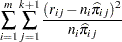
The Pearson chi-square statistic  and the deviance
  are given by
 |
 |
 |
|||
 |
|
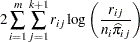 |
where  is the number of subpopulation profiles,
  is the number of response levels,
  is the total weight (sum of the product of the frequencies and the weights) associated with
  th level responses in the
  th profile,
  , and
, and  is the fitted probability for the th level at the th profile. Each of these chi-square statistics has
  degrees of freedom, where
  is the number of parameters estimated. The dispersion parameter is estimated by
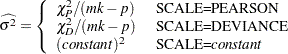 |
In order for the Pearson statistic and the deviance to be distributed as chi-square, there must be sufficient replication within the subpopulations. When this is not true, the data are sparse, and the p-values for these statistics are not valid and should be ignored. Similarly, these statistics, divided by their degrees of freedom, cannot serve as indicators of overdispersion. A large difference between the Pearson statistic and the deviance provides some evidence that the data are too sparse to use either statistic.
You can use the AGGREGATE (or AGGREGATE=) option to define the subpopulation profiles. If you do not specify this option, each observation is regarded as coming from a separate subpopulation. For events/trials syntax, each observation represents  Bernoulli trials, where is the value of the trials variable; for single-trial syntax, each observation represents a single trial. Without the AGGREGATE (or AGGREGATE=) option, the Pearson chi-square statistic and the deviance are calculated only for events/trials syntax.
Note that the parameter estimates are not changed by this method. However, their standard errors are adjusted for overdispersion, affecting their significance tests.
Williams’ Method
Suppose that the data consist of binomial observations. For the th observation, let  be the observed proportion and let
  be the associated vector of explanatory variables. Suppose that the response probability for the th observation is a random variable
  with mean and variance
 |
where  is the probability of the event, and
  is a nonnegative but otherwise unknown scale parameter. Then the mean and variance of
  are
are
 |
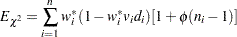
Williams (1982) estimates the unknown parameter by equating the value of Pearson’s chi-square statistic for the full model to its approximate expected value. Suppose  is the weight associated with the th observation. The Pearson chi-square statistic is given by
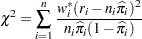 |
Let  be the first derivative of the link function
  . The approximate expected value of
  is
is
 |
where 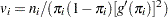 and
and  is the variance of the linear predictor
  . The scale parameter is estimated by the following iterative procedure.
At the start, let  and let
  be approximated by ,
  . If you apply these weights and approximated probabilities to and
  and then equate them, an initial estimate of is
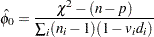 |
where is the total number of parameters. The initial estimates of the weights become 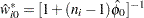 . After a weighted fit of the model, the
  and
and  are recalculated, and so is . Then a revised estimate of is given by
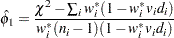 |
The iterative procedure is repeated until is very close to its degrees of freedom.
Once has been estimated by  under the full model, weights of
 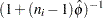 can be used to fit models that have fewer terms than the full model. See Example 51.10 for an illustration.
Note:If the WEIGHT statement is specified with the NORMALIZE option, then the initial values are set to the normalized weights, and the weights resulting from Williams’ method will not add up to the actual sample size. However, the estimated covariance matrix of the parameter estimates remains invariant to the scale of the WEIGHT variable.
Copyright © SAS Institute, Inc. All Rights Reserved.