Some Important PROC CALIS Features

Modeling Languages for Specifying Models

PROC CALIS provides several modeling languages to specify a model. Different modeling languages in PROC CALIS are signified by the main model specification statement used. In this chapter, you have seen examples of the FACTOR, LINEQS, LISMOD, MSTRUCT, PATH, and RAM modeling languages. Depending on your modeling philosophy and the type of the model, you can choose a modeling language that is most suitable for your application. For example, models specified using structural equations can be transcribed directly into the LINEQS statement. Models that are hypothesized using path diagrams can be described easily in the PATH or RAM statement. First-order confirmatory or exploratory factor models are most conveniently specified by using the FACTOR and MATRIX statements. Traditional LISREL models are supported through the LISMOD and MATRIX statements. Finally, patterned covariance and mean models can be specified directly by the MSTRUCT and MATRIX statements.

For most applications, the PATH and LINEQS statements are the easiest to use. In other cases, the FACTOR, LISMOD, MSTRUCT, or RAM statement might be more suitable. See the section Which Modeling Language? in Chapter 25, The CALIS Procedure, for a more detailed discussion.

For very general matrix model specifications, you can use the COSAN modeling language. See the COSAN statement and the section The COSAN Model of Chapter 25, The CALIS Procedure, for details.

Estimation Methods

The CALIS procedure provides six methods of estimation specified by the METHOD= option:

Each estimation method is based on finding parameter estimates that minimize a discrepancy (badness-of-fit) function, which measures the difference between the observed sample covariance matrix and the fitted (predicted) covariance matrix, given the model and the parameter estimates. See the section Estimation Criteria in Chapter 25, The CALIS Procedure, for formulas, or refer to Loehlin (1987, pp. 54–62) and Bollen (1989, pp. 104–123) for further discussion.

The default is METHOD=ML, which is the most popular method for applications. The option METHOD=GLS usually produces very similar results to those produced by METHOD=ML. If your data contain random missing values and it is important to use the information from those incomplete observations, you might want to use the FIML method, which provides a sound treatment of missing values in data. METHOD=ML and METHOD=FIML are essentially the same method when you do not have missing values (see Example 25.14). Asymptotically, ML and GLS are the same. Both methods assume a multivariate normal distribution in the population. The WLS method with the default weight matrix is equivalent to the asymptotically distribution free (ADF) method, which yields asymptotically normal estimates regardless of the distribution in the population. When the multivariate normal assumption is in doubt, especially if the variables have high kurtosis, you should seriously consider the WLS method. When a correlation matrix is analyzed, only WLS can produce correct standard error estimates. However, in order to use the WLS method with the expected statistical properties, the sample size must be large. Several thousand might be a minimum requirement.

The ULS and DWLS methods yield reasonable estimates under less restrictive assumptions. You can apply these methods to normal or nonnormal situations or to covariance or correlation matrices. The drawback is that the statistical qualities of the estimates seem to be unknown. For this reason, PROC CALIS does not provide standard errors or test statistics with these two methods.

You cannot use METHOD=ML or METHOD=GLS if the observed covariance matrix is singular. You can either remove variables involved in the linear dependencies or use less restrictive estimation methods such as ULS. Specifying METHOD=ML assumes that the predicted covariance matrix is nonsingular. If ML fails because of a singular predicted covariance matrix, you need to examine whether the model specification leads to the singularity. If so, modify the model specification to eliminate the problem. If not, you probably need to use other estimation methods.

You should remove outliers and try to transform variables that are skewed or heavy-tailed. This applies to all estimation methods, since all the estimation methods depend on the sample covariance matrix, and the sample covariance matrix is a poor estimator for distributions with high kurtosis (Bollen 1989, pp. 415–418; Huber 1981; Hampel et al. 1986). PROC CALIS displays estimates of univariate and multivariate kurtosis (Bollen; 1989, pp. 418–425) if you specify the KURTOSIS option in the PROC CALIS statement.

See the section Estimation Methods for the general use of these methods. See the section Estimation Criteria of Chapter 25, The CALIS Procedure, for details about these estimation criteria.

Statistical Inference

When you specify the ML, FIML, GLS, or WLS estimation with appropriate models, PROC CALIS can compute the following:

• a chi-square goodness-of-fit test of the specified model versus the alternative that the data are from a population with unconstrained covariance matrix (Loehlin 1987, pp. 62–64; Bollen 1989, pp. 110, 115, 263–269)

• approximate standard errors of the parameter estimates (Bollen; 1989, pp. 109, 114, 286), displayed with the STDERR option

• various modification indices, requested via the MODIFICATION or MOD option, that give the approximate change in the chi-square statistic that would result from removing constraints on the parameters or constraining additional parameters to zero (Bollen 1989, pp. 293–303)

If you have two models such that one model results from imposing constraints on the parameters of the other, you can test the constrained model against the more general model by fitting both models with PROC CALIS. If the constrained model is correct, the difference between the chi-square goodness of fit statistics for the two models has an approximate chi-square distribution with degrees of freedom equal to the difference between the degrees of freedom for the two models (Loehlin 1987, pp. 62–67; Bollen 1989, pp. 291–292).

All of the test statistics and standard errors computed under ML and GLS depend on the assumption of multivariate normality. Normality is a much more important requirement for data with random independent variables than it is for fixed independent variables. If the independent variables are random, distributions with high kurtosis tend to give liberal tests and excessively small standard errors, while low kurtosis tends to produce the opposite effects (Bollen; 1989, pp. 266–267, 415–432).

All test statistics and standard errors computed by PROC CALIS are based on asymptotic theory and should not be trusted in small samples. There are no firm guidelines on how large a sample must be for the asymptotic theory to apply with reasonable accuracy. Some simulation studies have indicated that problems are likely to occur with sample sizes less than 100 (Loehlin 1987, pp. 60–61; Bollen 1989, pp. 267–268). Extrapolating from experience with multiple regression would suggest that the sample size should be at least 5 to 20 times the number of parameters to be estimated in order to get reliable and interpretable results. The WLS method might even require that the sample size be over several thousand.

The asymptotic theory requires the parameter estimates to be in the interior of the parameter space. If you do an analysis with inequality constraints and one or more constraints are active at the solution (for example, if you constrain a variance to be nonnegative and the estimate turns out to be zero), the chi-square test and standard errors might not provide good approximations to the actual sampling distributions.

For modeling correlation structures, the only theoretically correct method is the WLS method with the default ASYCOV=CORR option. For other methods, standard error estimates for modeling correlation structures might be inaccurate even for sample sizes as large as 400. The chi-square statistic is generally the same regardless of which matrix is analyzed, provided that the model involves no scale-dependent constraints. However, if the purpose is to obtain reasonable parameter estimates for the correlation structures only, then you might also find other estimation methods useful.

If you fit a model to a correlation matrix and the model constrains one or more elements of the predicted matrix to equal 1.0, the degrees of freedom of the chi-square statistic must be reduced by the number of such constraints. PROC CALIS attempts to determine which diagonal elements of the predicted correlation matrix are constrained to a constant, but it might fail to detect such constraints in complicated models, particularly when programming statements are used. If this happens, you should add parameters to the model to release the constraints on the diagonal elements.

Multiple-Group Analysis

PROC CALIS supports multiple-group multiple-model analysis. You can fit the same covariance (and mean) structure model to several independent groups (data sets). Or, you can fit several different but constrained models to the independent groups (data sets). In PROC CALIS, you can use the GROUP statements to define several independent groups and the MODEL statements to define several different models. For example, the following statements show a multiple-group analysis by PROC CALIS:

proc calis;
   group 1 / data=set1;
   group 2 / data=set2;
   group 3 / data=set3;
   model 1 / group=1,2;
      path 
         y <--- x   = beta ,
         x <--- z   = gamma;
   model 2 / group=3;
      path   
         y <--- x   = beta,
         x <--- z   = alpha;
run;

In this specification, you conduct a three-group analysis. You define two PATH models. You fit Model 1 to Groups 1 and 2 and Model 2 to Group 3. The two models are constrained for the (y <- x) path because they use the same path coefficient parameter beta. Other parameters in the models are not constrained.

To facilitate model specification by model referencing, you can use the REFMODEL statement to specify models based on model referencing. For example, the previous example can be specified equivalently as the following statements:

proc calis;
   group 1 / data=set1;
   group 2 / data=set2;
   group 3 / data=set3;
   model 1 / group=1,2;
      path 
         y <--- x   = beta ,
         x <--- z   = gamma;
   model 2 / group=3;
      refmodel 1;
      renameparm gamma=alpha;   
run;

The current specification differs from the preceding specification in the definition of Model 2. In the current specification, Model 2 is making reference to Model 1. Basically, this means that the specification in Model 1 is transferred to Model 2. However, the RENAMEPARM statement requests a name change for gamma, which becomes a new parameter named alpha in Model 2. Hence, Model 2 and Model 1 are almost, but not exactly, the same. They are constrained by the same path coefficient beta for the (y <- x) path, but they have different path coefficients for the (x <- z) path.

Model referencing by the REFMODEL statement offers you an efficient and concise way to define models based on the similarities and differences between models. The advantages become more obvious when you have several large models in multiple-group analysis and each model differs just a little bit from each other.

Goodness-of-Fit Statistics

In addition to the chi-square test, there are many other statistics for assessing the goodness of fit of the predicted correlation or covariance matrix to the observed matrix.

Akaike’s information criterion (AIC, Akaike 1987) and Schwarz’s Bayesian criterion (SBC, Schwarz 1978) are useful for comparing models with different numbers of parameters—the model with the smallest value of AIC or SBC is considered best. Based on both theoretical considerations and various simulation studies, SBC seems to work better, since AIC tends to select models with too many parameters when the sample size is large.

There are many descriptive measures of goodness of fit that are scaled to range approximately from zero to one: the goodness-of-fit index (GFI) and GFI adjusted for degrees of freedom (AGFI) (Jöreskog and Sörbom; 1988), centrality (McDonald; 1989), and the parsimonious fit index (James, Mulaik, and Brett; 1982). Bentler and Bonett (1980) and Bollen (1986) have proposed measures for comparing the goodness of fit of one model with another in a descriptive rather than inferential sense.

The root mean squared error approximation (RMSEA) proposed by Steiger and Lind (1980) does not assume a true model being fitted to the data. It measures the discrepancy between the fitted model and the covariance matrix in the population. For samples, RMSEA and confidence intervals can be estimated. Statistical tests for determining whether the population RMSEAs fall below certain specified values are available (Browne and Cudeck; 1993). In the same vein, Browne and Cudeck (1993) propose the expected cross validation index (ECVI), which measures how good a model is for predicting future sample covariances. Point estimate and confidence intervals for ECVI are also developed.

None of these measures of goodness of fit are related to the goodness of prediction of the structural equations. Goodness of fit is assessed by comparing the observed correlation or covariance matrix with the matrix computed from the model and parameter estimates. Goodness of prediction is assessed by comparing the actual values of the endogenous variables with their predicted values, usually in terms of root mean squared error or proportion of variance accounted for (R square). For latent endogenous variables, root mean squared error and R square can be estimated from the fitted model.

Customizable Fit Summary Table

Because there are so many fit indices that PROC CALIS can display and researchers prefer certain sets of fit indices, PROC CALIS enables you to customize the set of fit indices to display. For example, you can use the following statement to limit the set of fit indices to display:

fitindex on(only) = [chisq SRMSR RMSEA AIC];

With this statement, only the model-fit chi-square, standardized root mean square residual, root mean square error of approximation, and Akaiki’s information criterion are displayed in your output. You can also save all your fit index values in an output data file by adding the OUTFIT= option in the FITINDEX statement. This output data file contains all available fit index values even if you have limited the set of fit indices to display in the listing output.

Standardized Solution

In many applications in social and behavioral sciences, measurement scales of variables are arbitrary. Although it should not be viewed as a universal solution, some researchers resort to the standardized solution for interpreting estimation results. PROC CALIS computes the standardized solutions for all models (except for COSAN) automatically. Standard error estimates are also produced for standardized solutions so that you can examine the statistical significance of the standardized estimates too.

However, equality or linear constraints on parameters are almost always set on the unstandardized variables. These parameter constraints are not preserved when the estimation solution is standardized. This would add difficulties in interpreting standardized estimates when your model is defined meaningfully with constraints on the unstandardized variables.

A general recommendation is to make sure your variables are measured on "comparable" scales (it does not necessarily mean that they are mean- and variance-standardized) for the analysis. But what makes different kinds of variables "comparable" is an ongoing philosophical issue.

Some researchers might totally abandon the concept of standardized solutions in structural equation modeling. If you prefer to turn off the standardized solutions in PROC CALIS, you can use the NOSTAND option in the PROC CALIS statement.

Testing Parametric Functions

Oftentimes, researchers might have a priori hypotheses about the parameters in their models. After knowing the model fit is satisfactory, they want to test those hypotheses under the model. PROC CALIS provides two statements for testing these kinds of hypotheses. The TESTFUNC statement enables you to test each parametric function separately, and the SIMTEST statement enables you to test parametric functions jointly (and separately). For example, assuming that effect1, effect2, effect3, and effect4 are parameters in your model, the following SIMTEST statement tests the joint hypothesis test1, which consists of two component hypotheses diff_effect and sum_effect:

SIMTEST  test1 = (diff_effect sum_ffect);
diff_effect = effect1 - effect2;
sum_effect  = effect3 + effect4;

To make test1 well-defined, each of the component hypotheses diff_effect and sum_effect is assumed to be defined as a parametric function by some SAS programming statements. In the specification, diff_effect represents the difference between effect1 and effect2, and sum_effect represents the sum of effect3 and effect4. Hence, the component hypotheses being tested are:

Effect Analysis

In structural equation modeling, effects from one variable to other variables can be direct or indirect. For example, in the following path diagram x has a direct effect on z in addition to an indirect effect on z via y:

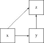
However, y has only a direct effect (but no indirect effect) on z. In cases like this, researchers are interested in computing the total, direct, and indirect effects from x and y to z. You can use the EFFPART option in the PROC CALIS statement to request this kind of effect partitioning in your model. Total, direct, and indirect effects are displayed, together with their standard error estimates. If your output contains standardized results (default), the standardized total, direct, and indirect effects and their standard error estimates are also displayed. With the EFFPART option, effects analysis is applied to all variables (excluding error terms) in your model.

In large models with many variables, researchers might want to analyze the effects only for a handful of variables. In this regard, PROC CALIS provides you a way to do a customized version of effect analysis. For example, the following EFFPART statement requests the effect partitioning of x1 and x2 on y1 and y2, even though there might be many more variables in the model:

 effpart   x1 x2 ---> y1 y2;

See the EFFPART statement of Chapter 25, The CALIS Procedure, for details.

Model Modifications

When you fit a model and the model fit is not satisfactory, you might want to know what you could do to improve the model. The LM (Lagrange multiplier) tests in PROC CALIS can help you improve the model fit by testing the potential free parameters in the model. To request the LM tests, you can use the MODIFICATION option in the PROC CALIS statement.

Usually, the LM test results contain lists of parameters, organized according to the types of parameters. In each list, the potential parameter with the greatest model improvement is shown first. Adding these new parameters improves the model fit approximately by the amount of the corresponding LM statistic.

Sometimes, researchers might have a target set of parameters they want to test in the LM tests. PROC CALIS offers a flexible way that you can customize the set the parameters for the LM tests. See the LMTESTS statement for details.

In addition, the Wald statistics produced by PROC CALIS suggest whether any parameters in your model can be dropped (or fixed to zero) without significantly affecting the model fit. You can request the Wald statistics with the MODIFICATION option in the PROC CALIS statement.

Optimization Methods

PROC CALIS uses a variety of nonlinear optimization algorithms for computing parameter estimates. These algorithms are very complicated and do not always work for every data set. PROC CALIS generally informs you when the computations fail, usually by displaying an error message about the iteration limit being exceeded. When this happens, you might be able to correct the problem simply by increasing the iteration limit (MAXITER= and MAXFUNC=). However, it is often more effective to change the optimization method (OMETHOD=) or initial values. For more details, see the section Use of Optimization Techniques in Chapter 25, The CALIS Procedure, and refer to Bollen (1989, pp. 254–256).

PROC CALIS might sometimes converge to a local optimum rather than the global optimum. To gain some protection against local optima, you can run the analysis several times with different initial estimates. The RANDOM= option in the PROC CALIS statement is useful for generating a variety of initial estimates.

Other Commonly Used Options

Other commonly used options in the PROC CALIS statement include the following:

• INMODEL= to input model specification from a data set, usually created by the OUTMODEL= option

• MEANSTR to analyze the mean structures

• NOBS to specify the number of observations

• NOPARMNAME to suppress the printing of parameter names

• NOSE to suppress the display of approximate standard errors

• OUTMODEL= to output model specification and estimation results to an external file for later use (for example, fitting the same model to other data sets)

• RESIDUAL to display residual correlations or covariances