ULS, GLS, and ML Discrepancy Functions

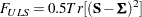
In each estimation method, the parameter vector is estimated iteratively by a nonlinear optimization algorithm that minimizes a discrepancy function , which is also known as the fit function in the literature. With denoting the number of manifest variables, the sample covariance matrix for a sample with size , the vector of sample means, the fitted covariance matrix, and the vector of fitted means, the discrepancy function for unweighted least squares (ULS) estimation is:

The discrepancy function for generalized least squares estimation (GLS) is:

By default, is assumed so that is the normal theory generalized least squares discrepancy function.

The discrepancy function for normal-theory maximum likelihood estimation (ML) is:

In each of the discrepancy functions, and are considered to be given and and are functions of model parameter vector . That is:

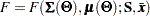Estimating by using a particular estimation method amounts to choosing a vector that minimizes the corresponding discrepancy function .

When the mean structures are not modeled or when the mean model is saturated by parameters, the last term of each fit function vanishes. That is, they become:

If, instead of being a covariance matrix, is a correlation matrix in the discrepancy functions, would naturally be interpreted as the fitted correlation matrix. Although whether is a covariance or correlation matrix makes no difference in minimizing the discrepancy functions, correlational analyses that use these functions are problematic because of the following issues:

• The diagonal of the fitted correlation matrix might contain values other than ones, which violates the requirement of being a correlation matrix.

• Whenever available, standard errors computed for correlation analysis in PROC CALIS are straightforward generalizations of those of covariance analysis. In very limited cases these standard errors are good approximations. However, in general they are not even asymptotically correct.

• The model fit chi-square statistic for correlation analysis might not follow the theoretical distribution, thus making model fit testing difficult.

Despite these issues in correlation analysis, if your primary interest is to obtain the estimates in the correlation models, you might still find PROC CALIS results for correlation analysis useful.

The statistical techniques used in PROC CALIS are primarily developed for the analysis of covariance structures, and hence COVARIANCE is the default option. Depending on the nature of your research, you can add the mean structures in the analysis by specifying mean and intercept parameters in your models. However, you cannot analyze mean structures simultaneously with correlation structures (see the CORRELATION option) in PROC CALIS.

FIML Discrepancy Function

The full information maximum likelihood method (FIML) assumes multivariate normality of the data. Suppose that you analyze a model that contains observed variables. The discrepancy function for FIML is

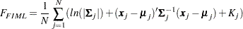where is a data vector for observation , and is a constant term (to be defined explicitly later) independent of the model parameters . In the current formulation, ’s are not required to have the same dimensions. For example, could be a complete vector with all variables present while is a vector with one missing value that has been excluded from the original data vector. As a consequence, subscript is also used in and to denote the submatrices that are extracted from the entire structured mean vector () and covariance matrix (). In other words, in the current formulation and do not mean that each observation is fitted by distinct mean and covariance structures (although theoretically it is possible to formulate FIML in such a way). The notation simply signifies that the dimensions of and of the associated mean and covariance structures could vary from observation to observation.

Let be the number of variables without missing values for observation . Then denotes a data vector, denotes a vector of means (structured with model parameters), is a matrix for variances and covariances (also structured with model parameters), and is defined by the following formula, which is a constant term independent of model parameters:

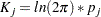As a general estimation method, the FIML method is based on the same statistical principle as the ordinary maximum likelihood (ML) method for multivariate normal data—that is, both methods maximize the normal theory likelihood function given the data. In fact, used in PROC CALIS is related to the log-likelihood function by the following formula:

Because the FIML method can deal with observations with various levels of information available, it is primarily developed as an estimation method that could deal with data with random missing values. See the section Relationships among Estimation Criteria for more details about the relationship between FIML and ML methods.

Whenever you use the FIML method, the mean structures are automatically assumed in the analysis. This is due to fact that there is no closed-form formula to obtain the saturated mean vector in the FIML discrepancy function if missing values are present in the data. You can certainly provide explicit specification of the mean parameters in the model by specifying intercepts in the LINEQS statement or means and intercepts in the MEAN or MATRIX statement. However, usually you do not need to do the explicit specification if all you need to achieve is to saturate the mean structures with parameters (that is, the same number as the number of observed variables in the model). With METHOD=FIML, PROC CALIS uses certain default parameterizations for the mean structures automatically. For example, all intercepts of endogenous observed variables and all means of exogenous observed variables are default parameters in the model, making the explicit specification of these mean structure parameters unnecessary.

WLS and ADF Discrepancy Functions

Another important discrepancy function to consider is the weighted least squares (WLS) function. Let be a vector containing all nonredundant elements in the sample covariance matrix and sample mean vector , with representing the vector of the lower triangle elements of the symmetric matrix , stacking row by row. Similarly, let be a vector containing all nonredundant elements in the fitted covariance matrix and the fitted mean vector , with representing the vector of the lower triangle elements of the symmetric matrix .

The WLS discrepancy function is:

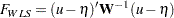where is a positive definite symmetric weight matrix with rows and columns. Because is a function of model parameter vector under the structural model, you can write the WLS function as:

Suppose that converges to with increasing sample size, where and denote the population covariance matrix and mean vector, respectively. By default, the WLS weight matrix in PROC CALIS is computed from the raw data as a consistent estimate of the asymptotic covariance matrix of , with partitioned as

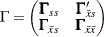where denotes the asymptotic covariance matrix for , denotes the asymptotic covariance matrix for , and denotes the 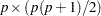asymptotic covariance matrix between and .

To compute the default weight matrix as a consistent estimate of , define a similar partition of the weight matrix as:

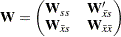Each of the submatrices in the partition can now be computed from the raw data. First, define the biased sample covariance for variables and as:

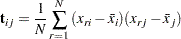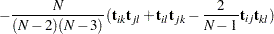
and the sample fourth-order central moment for variables , , , and as:

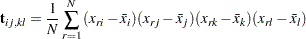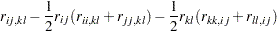
The submatrices in are computed by:

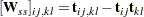Assuming the existence of finite eighth-order moments, this default weight matrix is a consistent but biased estimator of the asymptotic covariance matrix .

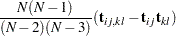
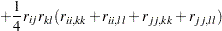
By using the ASYCOV= option, you can use Browne’s unbiased estimator (Browne; 1984, formula (3.8)) of as:

There is no guarantee that computed this way is positive semidefinite. However, the second part is of order and does not destroy the positive semidefinite first part for sufficiently large . For a large number of independent observations, default settings of the weight matrix result in asymptotically distribution-free parameter estimates with unbiased standard errors and a correct test statistic (Browne; 1982, 1984).

With the default weight matrix computed by PROC CALIS, the WLS estimation is also called as the asymptotically distribution-free (ADF) method. In fact, as options in PROC CALIS, METHOD=WLS and METHOD=ADF are totally equivalent, even though WLS in general might include cases with special weight matrices other than the default weight matrix.

When the mean structures are not modeled, the WLS discrepancy function is still the same quadratic form statistic. However, with only the elements in covariance matrix being modeled, the dimensions of and are both reduced to , and the dimension of the weight matrix is now . That is, the WLS discrepancy function for covariance structure models is:

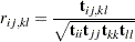
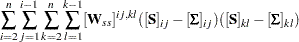
If is a correlation rather than a covariance matrix, the default setting of the is a consistent estimator of the asymptotic covariance matrix of (Browne and Shapiro; 1986; DeLeeuw; 1983), with and representing vectors of sample and population correlations, respectively. Elementwise, is expressed as:

where

and

The asymptotic variances of the diagonal elements of a correlation matrix are 0. That is,

for all . Therefore, the weight matrix computed this way is always singular. In this case, the discrepancy function for weighted least squares estimation is modified to:

where is the penalty weight specified by the WPENALTY= option and the are the elements of the inverse of the reduced weight matrix that contains only the nonzero rows and columns of the full weight matrix .

The second term is a penalty term to fit the diagonal elements of the correlation matrix . The default value of can be decreased or increased by the WPENALTY= option. The often used value of seems to be too small in many cases to fit the diagonal elements of a correlation matrix properly.

Note that when you model correlation structures, no mean structures can be modeled simultaneously in the same model.

DWLS Discrepancy Functions

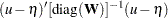
Storing and inverting the huge weight matrix in WLS estimation requires considerable computer resources. A compromise is found by implementing the diagonally weighted least squares (DWLS) method that uses only the diagonal of the weight matrix from the WLS estimation in the following discrepancy function:

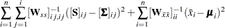When only the covariance structures are modeled, the discrepancy function becomes:

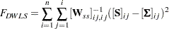For correlation models, the discrepancy function is:

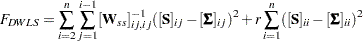where is the penalty weight specified by the WPENALTY= option. Note that no mean structures can be modeled simultaneously with correlation structures when using the DWLS method.

As the statistical properties of DWLS estimates are still not known, standard errors for estimates are not computed for the DWLS method.

Input Weight Matrices

In GLS, WLS, or DWLS estimation you can change from the default settings of weight matrices by using an INWGT= data set. The CALIS procedure requires a positive definite weight matrix that has positive diagonal elements.

Multiple-Group Discrepancy Function

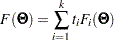
Suppose that there are independent groups in the analysis and , , ..., are the sample sizes for the groups. The overall discrepancy function is expressed as a weighted sum of individual discrepancy functions ’s for the groups:

where

is the weight of the discrepancy function for group , and

is the total number of observations in all groups. In PROC CALIS, all discrepancy function ’s in the overall discrepancy function must belong to the same estimation method. You cannot specify different estimation methods for the groups in a multiple-group analysis. In addition, the same analysis type must be applied to all groups—that is, you can analyze either covariance structures, covariance and mean structures, and correlation structures for all groups.