Example 95.4 Covariogram and Semivariogram

The covariance that was reviewed in the section Stationarity is an alternative measure of spatial continuity that can be used instead of the semivariance. In a similar manner to the empirical semivariance that was presented in the section Theoretical and Computational Details of the Semivariogram, you can also compute the empirical covariance. The covariograms are plots of this quantity and can be used to fit permissible theoretical covariance models, in correspondence to the semivariogram analysis presented in the section Theoretical Semivariogram Models. This example displays a comparative view of the empirical covariogram and semivariogram, and examines some additional aspects of these two measures.

You consider 500 simulations of an SRF in a square domain of ( km). The following DATA step defines the data locations:

   title 'Covariogram and Semivariogram Example';
   data dataCoord;
      retain seed 837591;
      do i=1 to 100;
         East = round(100*ranuni(seed),0.1);
         North = round(100*ranuni(seed),0.1);
         output;
      end;
   run;

For the simulations you use PROC SIM2D, which produces Gaussian simulations of SRFs with user-specified covariance structure—see Chapter 79, The SIM2D Procedure. The Gaussian SRF implies full knowledge of the SRF expected value and variance at every location . The following statements simulate an isotropic, second-order stationary SRF with constant expected value and variance throughout the simulation domain:

   ods graphics on;

   proc sim2d outsim=dataSims; 
      simulate numreal=500 seed=79750 
               nugget=2 scale=6 range=10 form=exp; 
      mean 30;
      grid gdata=dataCoord xc=East yc=North; 
   run; 

Here, the SIMULATE statement accommodates the simulation parameters. The NUMREAL= option specifies that you want to perform 500 simulations, and the SEED= option specifies the seed for the simulation random number generator. You use the MEAN statement to specify the expected value units of . You also specify two variance components. The first is the nugget effect, and you use the NUGGET= option to set it to . The second is the partial sill that you specify with the SCALE= option. The two variance components make up the total SRF variance . You assume an exponential covariance structure to describe the field spatial continuity, where is the sill value, and its range km (effective range km) is specified by the RANGE= option. The option FORM= specifies the covariance structure type.

The empirical semivariance and covariance are computed by the VARIOGRAM procedure, and are available either in the ODS output semivariogram table (as variables Semivariance and Covariance, respectively) or in the OUTVAR= data set. In the following statements you obtain these variables by using the OUTVAR= data set of the VARIOGRAM procedure:

   proc variogram data=dataSims outv=outv noprint;
      compute lagd=3 maxlag=18;
      coord xc=gxc yc=gyc;
      by _ITER_;
      var svalue;
   run;

For each distance lag you take the average of the empirical measures over the number of simulations. PROC SORT is used to prepare the input data for PROC MEANS, which produces these averages and stores them in the dataAvgs data set. This sequence is performed with the following statements:

   proc sort data=outv;
      by lag;
   run;

   proc means data=outv n mean noprint;
      var Distance variog covar;
      by lag; 
      output out=dataAvgs mean(variog)=Semivariance
                          mean(covar)=Covariance
                          mean(Distance)=Distance; 
   run;

The SGPLOT procedure is used to create the plot of the average empirical semivariogram and covariogram, as in the following statements:

   proc sgplot data=dataAvgs;
      title "Empirical Semivariogram and Covariogram";
      xaxis label = "Distance" grid;
      yaxis  label = "Semivariance" min=-0.5 max=9 grid;
      y2axis label = "Covariance"   min=-0.5 max=9;
      scatter y=Semivariance x=Distance /
              markerattrs = GraphData1
              name='Semivar'
              legendlabel='Semivariance';
      scatter y=Covariance x=Distance /
              y2axis
              markerattrs = GraphData2
              name='Covar'
              legendlabel='Covariance';
      discretelegend 'Semivar' 'Covar';
   run; 
   
   ods graphics off;

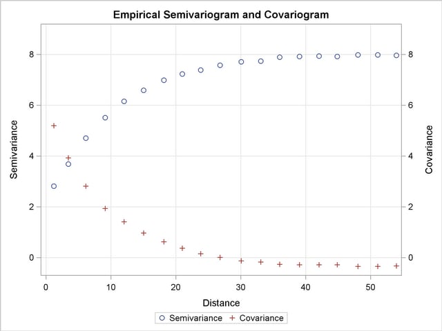
The plot of the average empirical semivariance and covariance of the preceding analysis is shown in Output 95.4.1. Note that the high number of simulations led to averages of empirical continuity measures that accurately approximate the simulated SRF characteristics. Specifically, the empirical semivariogram and covariogram both exhibit clearly exponential behavior. The semivariogram sill is approximately at the specified variance of the SRF.

The simulated SRF is second-order stationary, so you expect at each lag the sum of the empirical semivariance and covariance to approximate the field variance , as explained in the section Stationarity. This behavior is evident in Output 95.4.1.

We conclude with a discussion of basic reasons why the empirical semivariogram analysis is commonly preferred to the empirical covariance analysis. A first reason comes from the assumptions that are necessary to compute each of these two measures. The condition of intrinsic stationarity that is required in order to define the empirical semivariogram is less restrictive than the condition of second-order stationarity that is required in order to consider the covariance function as a parameter of the process.

Also, an empirical semivariogram can indicate whether a nugget effect is present in your data sample, whereas the empirical covariogram itself might not reveal this information. This point is illustrated in Output 95.4.1, where you expect to see that , but the empirical covariogram cannot have a point at exactly . There is a practical way to investigate for a nugget effect when you use empirical covariograms. Recall that the OUTVAR= data set provides you with the sample variance (shown in the COVAR column for LAG=), as the following statement shows:

   /* Obtain the sample variance from the data set ----------------*/
   
   proc print data=dataAvgs (obs=1);

Output 95.4.1 Average Empirical Semivariogram and Covariogram from 500 Simulations

Output 95.4.2 is a partial output of the dataAvgs data set, which contains averages of the OUTVAR= data set, and shows the computed average in the Covariance column. The combination of the empirical covariogram and the value can help you fit a theoretical covariance model that will include any nugget effect, if present. See also the discussion in Schabenberger and Gotway (2005, Section 4.2.2) about the Matérn definition of the covariance function that is related to this issue. In particular, this definition provides for an additional variance component in the covariance expression at to account for the corresponding nugget effect in the semivariogram.

In addition to the preceding points, if the SRF is nonstationary, the empirical semivariogram indicates that the SRF variance will increase with distance , as Output 95.3.1 shows in Analysis without Surface Trend Removal. In that case it makes no sense to compute the empirical covariogram. Specifically, the covariogram could provide you with an estimate of the sample variance, which is not sufficient to indicate that the SRF might not be stationary (see also Chilès and Delfiner; 1999, p. 31).

Finally, the definitions of the empirical semivariance and covariance in the section Theoretical and Computational Details of the Semivariogram clearly show that the sample mean and the SRF expected value are not important for the computation of the semivariance, but either one is necessary for the covariance. Hence, the semivariance expression filters the mean, which is especially useful when it is unknown. On the other hand, if is unknown and the empirical covariance is computed based on the sample mean , this can induce additional bias in the covariance computation.