| The TCALIS Procedure |
Example 88.3 A Direct Covariance Structures Model
In the section Direct Covariance Structures Analysis, the MSTRUCT modeling language is used to specify a model with direct covariance structures. In the model, four variables from the data set of Wheaton et al. (1977) are used. The analysis is carried out in this example to investigate the tenability of the hypothesized covariance structures.
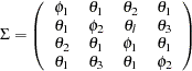
The four variables used are: Anomie67, Powerless67, Anomie71, and Powerless71. The hypothesized covariance matrix is structured as:
 |
where:
 :
:variance of anomie
 :
:variance of powerlessness
 :
:covariance between anomie and powerlessness
 :
:covariance between anomie measures
 :
:covariance between powerlessness measures
In this example, you hypothesize the covariance structures directly, as opposed to those models with implied covariance structures from path models (see Example 88.1), structural equations (see Example 88.2), or other types of models. The basic assumption of the direct covariance structures in this example is that Anomie and Powerless were invariant over the measurement periods employed. This implies that the time of measurement did not change the variances and covariances of the measures. Therefore, both Anomie67 and Anomie71 have the same variance parameter , and both Powerless67 and Powerless71 have the same variance parameter . These two parameters, and , are hypothesized on the diagonal of the covariance matrix  . In the same structured covariance matrix, represents the covariance between Anomie and Powerless, without regard to the time of measurement. The parameter represents the covariance between the Anomie measures, or the reliability of the Anomie measure. Similarly, the parameter represents the covariance between the Powerless measures, or the reliability of the Anomie measure.
As explained in the section Direct Covariance Structures Analysis, you can use the MSTRUCT modeling language to specify the hypothesized covariance structures directly, as shown in the following statements:
   proc tcalis nobs=932 data=Wheaton psummary;
      fitindex on(only)=[chisq df probchi] outfit=savefit;
      mstruct
         var = Anomie67 Powerless67 Anomie71 Powerless71;
      matrix _COV_ [1,1] = phi1,
                   [2,2] = phi2,
                   [3,3] = phi1,
                   [4,4] = phi2,
                   [2,1] = theta1,
                   [3,1] = theta2,
                   [3,2] = theta1,
                   [4,1] = theta1,
                   [4,2] = theta3,
                   [4,3] = theta1;
   run;
In the MSTRUCT statement you specify the variables in the VAR= list. The order of variables in this VAR= list is assumed to be the same as that in the row and column of the hypothesized covariance matrix. Next, in the MATRIX statement you specify parameters as entries in the hypothesized covariance matrix _COV_. Only the lower diagonal elements need to be specified because covariance matrices, by nature, are symmetric. Redundant specification of the upper triangular elements are unnecessary as PROC TCALIS has the information accounted for. You can also set initial estimates by putting parenthesized numbers after the parameter names. But in this example you let PROC TCALIS determine all the initial estimates.
In the PROC TCALIS statement, the PSUMMARY option is used. As a global display option, this option suppresses a lot of displayed output and requests only the fit summary table be printed. This way you can eliminate quite a lot of displayed output that is not of your primary interest. In this example, the specification of the covariance structures is straightforward, and you do not need any output regarding the initial estimation or standardized solution. Suppose that you are not even concerned with the estimates of the parameters because you are not yet sure if this model is good enough for the data. All you want to know at this stage is whether the hypothesized covariance structures fit the data well. Therefore, the PSUMMARY option would serve your purpose well in this example.
In fact, even the fit summary table can be trimmed down quite a bit if you only want to look at certain specific fit indices. In the FITINDEX statement of this example, the ON(ONLY)= option turns on the printing of the model fit chi-square, its  , and
, and  -value only. This does not mean that you must lose the information of all other fit indices. In addition to the printed output, you can save all fit indices in an output data set. To this end, you can use the OUTFIT= option in the FITINDEX statement. In this example, you save the results of all fit indices in a SAS data set called savefit.
The entire printed output is shown in Output 88.3.1.
As you can see, the displayed output is very precise. It contains only a fit summary table with three statistics. The -value for the mode fit chi-square test indicates that the hypothesized structures should be rejected at  . Therefore, this rather restrictive direct covariance structure model does not fit the data well. A less restrictive covariance structure model with more parameters is needed to better account for the variances and covariances of the variables.
All fit indices are saved in the savefit data set. To view it, you can use the following statement:
   proc print data=savefit;
   run;
All indices, their types and values are shown in Output 88.3.2.
| Analysis of Direct Covariance Structures |
| Testing Model by the MSTRUCT Language |
| Obs | _TYPE_ | FitIndex | FitValue | PrintChar |
|---|---|---|---|---|
| 1 | ModelInfo | N Observations | 932.00 | 932 |
| 2 | ModelInfo | N Variables | 4.00 | 4 |
| 3 | ModelInfo | N Moments | 10.00 | 10 |
| 4 | ModelInfo | N Parameters | 5.00 | 5 |
| 5 | ModelInfo | N Active Constraints | 0.00 | 0 |
| 6 | ModelInfo | Independence Model Chi-Square | 1563.94 | 1563.9442 |
| 7 | ModelInfo | Independence Model Chi-Square DF | 6.00 | 6 |
| 8 | Absolute | Fit Function | 0.24 | 0.2380 |
| 9 | Absolute | Chi-Square | 221.58 | 221.5798 |
| 10 | Absolute | Chi-Square DF | 5.00 | 5 |
| 11 | Absolute | Pr > Chi-Square | 0.00 | 0.0000 |
| 12 | Absolute | Elliptic Corrected Chi-Square | . | . |
| 13 | Absolute | Pr > Elliptic Corr. Chi-Square | . | . |
| 14 | Absolute | Z-Test of Wilson & Hilferty | 12.25 | 12.2533 |
| 15 | Absolute | Hoelter Critical N | 48.00 | 48 |
| 16 | Absolute | Root Mean Square Residual (RMSR) | 0.76 | 0.7649 |
| 17 | Absolute | Standardized RMSR (SRMSR) | 0.07 | 0.0701 |
| 18 | Absolute | Goodness of Fit Index (GFI) | 0.90 | 0.9036 |
| 19 | Parsimony | Adjusted GFI (AGFI) | 0.81 | 0.8071 |
| 20 | Parsimony | Parsimonious GFI | 0.75 | 0.7530 |
| 21 | Parsimony | RMSEA Estimate | 0.22 | 0.2157 |
| 22 | Parsimony | RMSEA Lower 90% Confidence Limit | 0.19 | 0.1920 |
| 23 | Parsimony | RMSEA Upper 90% Confidence Limit | 0.24 | 0.2404 |
| 24 | Parsimony | Probability of Close Fit | 0.00 | 0.0000 |
| 25 | Parsimony | ECVI Estimate | 0.25 | 0.2488 |
| 26 | Parsimony | ECVI Lower 90% Confidence Limit | 0.20 | 0.2003 |
| 27 | Parsimony | ECVI Upper 90% Confidence Limit | 0.31 | 0.3053 |
| 28 | Parsimony | Akaike Information Criterion | 211.58 | 211.5798 |
| 29 | Parsimony | Bozdogan CAIC | 182.39 | 182.3932 |
| 30 | Parsimony | Schwarz Bayesian Criterion | 187.39 | 187.3932 |
| 31 | Parsimony | McDonald Centrality | 0.89 | 0.8903 |
| 32 | Incremental | Bentler Comparative Fit Index | 0.86 | 0.8610 |
| 33 | Incremental | Bentler-Bonett NFI | 0.86 | 0.8583 |
| 34 | Incremental | Bentler-Bonett Non-normed Index | 0.83 | 0.8332 |
| 35 | Incremental | Bollen Normed Index Rho1 | 0.83 | 0.8300 |
| 36 | Incremental | Bollen Non-normed Index Delta2 | 0.86 | 0.8611 |
| 37 | Incremental | James et al. Parsimonious NFI | 0.72 | 0.7153 |
The results of various fit indices from this output data set confirm that the hypothesized model does not fit the data well.
As an aside, it is noted with some shorthand notation, the specification of the MSTRUCT model parameters that use the MATRIX statements can be made a little more precise for the current example. This is shown as follows:
   proc tcalis nobs=932 data=Wheaton psummary;
      fitindex on(only)=[chisq df probchi] outfit=savefit;
      mstruct
         var = Anomie67 Powerless67 Anomie71 Powerless71;
      matrix _COV_ [1,1] = phi1 phi2 phi1 phi2;
                   [2, ] = theta1,
                   [3, ] = theta2 theta1,
                   [4, ] = theta1 theta3 theta1;
   run;
In the first entry of the MATRIX statement, the notation [1,1] represents that the parameter list specified after the equal sign starts with the [1,1] element of the _COV_ matrix and proceeds down the diagonal. In the next three entries, the notations [2,], [3,], and [4,] represent that parameter lists start with the first elements of the second, third, and fourth rows, respectively, and proceed to the next (right) elements on the same rows. See the syntax of the MATRIX statement for more details about this kind of shorthand notation.
Note: This procedure is experimental.
Copyright © 2009 by SAS Institute Inc., Cary, NC, USA. All rights reserved.