| The TCALIS Procedure |
Example 88.2 Simultaneous Equations with Mean Structures and Reciprocal Paths
The supply-and-demand food example of Kmenta (1971, pp. 565, 582) is used to illustrate PROC TCALIS for the estimation of intercepts and coefficients of simultaneous equations in econometrics. The model is specified by two simultaneous equations containing two endogenous variables  and
and  , and three exogenous variables
  ,
,  , and
, and  :
:
 |
 |
for  , ...,
  .
.
To analyze this model in PROC TCALIS, the second equation needs to be written in another form. For instance, in the LINEQS model each endogenous variable must appear on the left-hand side of exactly one equation. To satisfy this requirement, you can rewrite the second equation as an equation for  as:
as:
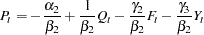 |
or, equivalently reparameterized as:
 |
where
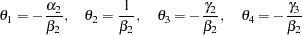 |
This new equation for together with the first equation for  suggest the following LINEQS model specification in PROC TCALIS:
   title 'Food example of KMENTA(1971, p.565 & 582)';
   data food;
     input Q P D F Y;
     label  Q='Food Consumption per Head'
            P='Ratio of Food Prices to General Price'
            D='Disposable Income in Constant Prices'
            F='Ratio of Preceding Years Prices'
            Y='Time in Years 1922-1941';
   datalines;
     98.485  100.323   87.4   98.0   1
     99.187  104.264   97.6   99.1   2
    102.163  103.435   96.7   99.1   3
    101.504  104.506   98.2   98.1   4
    104.240   98.001   99.8  110.8   5
    103.243   99.456  100.5  108.2   6
    103.993  101.066  103.2  105.6   7
     99.900  104.763  107.8  109.8   8
    100.350   96.446   96.6  108.7   9
    102.820   91.228   88.9  100.6  10
     95.435   93.085   75.1   81.0  11
     92.424   98.801   76.9   68.6  12
     94.535  102.908   84.6   70.9  13
     98.757   98.756   90.6   81.4  14
    105.797   95.119  103.1  102.3  15
    100.225   98.451  105.1  105.0  16
    103.522   86.498   96.4  110.5  17
     99.929  104.016  104.4   92.5  18
    105.223  105.769  110.7   89.3  19
    106.232  113.490  127.1   93.0  20
   ;
   proc tcalis data=food pshort nostand;
      lineqs
         Q = alpha1 Intercept + beta1  P  + gamma1 D + E1,
         P = theta1 Intercept + theta2 Q  + theta3 F + theta4 Y + E2;
      std
         E1-E2 = eps1-eps2;
      cov
         E1-E2 = eps3;
      bounds
         eps1-eps2 >= 0. ;
   run;
The LINEQS modeling language is used in this example because its specification is similar to the original equations. In the LINEQS statement, you essentially input the two model equations for Q and P. Parameters for intercepts and regression coefficients are also specified in the equations. Note that Intercept in the two equations is treated as a special variable that contains ones for all observations. Intercept is not a variable in the data set, nor do you need to create such a variable in your data set. Hence, the variable Intercept does not represent the intercept parameter itself. Instead, the intercept parameters for the two equations are the coefficients attached to Intercept. In this example, the intercept parameters are alpha1 and theta1, respectively, in the two equations. As required, error terms E1 and E2 are added to complete the equation specification.
In the STD statement, you specify eps1 and eps2, respectively, for the variance parameters of the error terms. In the COV, you specify eps3 for the covariance parameter between the error terms. In the BOUNDS statement, you set lower bounds for the error variances so that estimates of eps1 and eps2 would be nonnegative.
In this example, the PSHORT and the NOSTAND options are used in the PROC TCALIS statement. The PSHORT option suppresses a large amount of the output. For example, initial estimates are not printed and simple descriptive statistics and standard errors are not computed. The NOSTAND option suppresses the printing of the standardized results. Because the default printing in PROC TCALIS might produce a large amount of output, using these printing options make your output more concise and readable. Whenever appropriate, it is recommended that you consider using these printing options.
The estimated equations are shown in Output 88.2.1.
| Linear Equations | |||||||||||||||||||||
|---|---|---|---|---|---|---|---|---|---|---|---|---|---|---|---|---|---|---|---|---|---|
| Q | = | 93.6193 | * | Intercept | + | -0.2295 | * | P | + | 0.3100 | * | D | + | 1.0000 | E1 | ||||||
| Std Err | 7.5748 | alpha1 | 0.0923 | beta1 | 0.0448 | gamma1 | |||||||||||||||
| t Value | 12.3592 | -2.4856 | 6.9186 | ||||||||||||||||||
| P | = | -218.9 | * | Intercept | + | 4.2140 | * | Q | + | -0.9305 | * | F | + | -1.5579 | * | Y | + | 1.0000 | E2 | ||
| Std Err | 137.7 | theta1 | 1.7540 | theta2 | 0.3960 | theta3 | 0.6650 | theta4 | |||||||||||||
| t Value | -1.5897 | 2.4025 | -2.3500 | -2.3429 | |||||||||||||||||
The estimates of intercepts and regression coefficients are shown directly in the equations. Any number in an equation followed by an asterisk is an estimate. For the estimates in equations, the parameter names are shown underneath the associated variables. Any number in an equation not followed by an asterisk is a fixed value. For example, the value  attached to the error term in each of the output equation is fixed. Also, for fixed coefficients there are no parameter names underneath the associated variables.
All but the intercept estimates in the equation for predicting P are statistically significant at  (when using an approximate critical value of 2). The
  ratio for theta1 is
  , which implies that this intercept might have been zero in the population. However, because you have reparameterized the original model to use the LINEQS model specification, transformed parameters like theta1 in this model might not be of primary interest. Therefore, you might not need to pay any attention to the significance of the theta1 estimate. There is a way to use the original econometric parameters to specify the LINEQS model. It is discussed in the later part of this example.
Estimates for variance, covariance, and mean parameters are shown in Output 88.2.2.
| Estimates for Variances of Exogenous Variables | |||||
|---|---|---|---|---|---|
| Variable Type |
Variable | Parameter | Estimate | Standard Error |
t Value |
| Error | E1 | eps1 | 3.51274 | 1.20204 | 2.92233 |
| E2 | eps2 | 105.06749 | 83.89446 | 1.25238 | |
| Observed | D | _Add1 | 139.96029 | 45.40911 | 3.08221 |
| F | _Add2 | 161.51355 | 52.40192 | 3.08221 | |
| Y | _Add3 | 35.00000 | 11.35550 | 3.08221 | |
Parameters with a name prefix _Add are added automatically by PROC TCALIS. These parameters are added as free parameters to complete the model specification. In PROC TCALIS, variances and covariances among the set of exogenous manifest variables must be parameters. You either specify them explicitly or let the TCALIS procedure to add them. If you need to constrain or to fix these parameters, then you must specify them explicitly. When your model also fits the mean structures, the same principle applies to the means of the exogenous manifest variables. In this example, because variables D, F, and Y are all exogenous manifest variables, their associated means, variances and covariances must be parameters in the model.
The squared multiple correlations for the equations are shown in Output 88.2.3.
For endogenous variable P, the R-square is  , which is obviously an invalid value. In fact, because there are correlated errors (between E1 and E2) and reciprocal paths (paths to and from Q and P), the model departs from the regular assumptions of multiple regression analysis. As a result, you should not interpret the R-squares for this example.
If you are interested in estimating the parameters in the original econometric model (that is,  ,
,  ,
,  , and
, and  ), the previous reparameterized LINEQS model does not serve your purpose well enough. However, using the relations between these original parameters with the
  parameters in the reparameterized LINEQS model, you can set up some "super-parameters" in the LINEQS model as follows:
   proc tcalis data=Food pshort nostand;
      lineqs
         Q = alpha1 Intercept + beta1  P  + gamma1 D + E1,
         P = theta1 Intercept + theta2 Q  + theta3 F + theta4 Y + E2;
      std
         E1-E2 = eps1-eps2;
      cov
         E1-E2 = eps3;
      bounds
         eps1-eps2 >= 0. ;
      parameters alpha2 (50.) beta2 gamma2 gamma3 (3*.25);
         theta1  = -alpha2 / beta2;
         theta2  = 1 / beta2;
         theta3  = -gamma2 / beta2;
         theta4  = -gamma3 / beta2;
   run;
In this new specification, only the PARAMETERS statement and the SAS programming statements following it are new. In the PARAMETERS statement, you define super-parameters alpha2, beta2, gamma2, and gamma3, and put initial values for them in parentheses. These parameters are the original econometric parameters of interest. The SAS programming statements that follow the PARAMETERS statement are used to define the functional relationships of the super-parameters with the parameters in the LINEQS model. Consequently, in this new specification, theta1, theta2, theta3, and theta4 are no longer independent parameters in the model, as they are in the previous reparameterized model. Instead, alpha2, beta2, gamma2, and gamma3 are independent parameters in this new specification. By fitting this new model, you get the same set of estimates as those in the previous LINEQS model. In addition, you get estimates of the super-parameters, as shown in Output 88.2.4.
You can now interpret the results in terms of the original econometric parameterization. As shown in Output 88.2.4, all these estimates are significant, despite the fact that one of the transformed parameter estimates in the linear equations of the LINEQS model is not. You can obtain almost equivalent results by applying the SAS/ETS procedure SYSLIN on this problem.
Note: This procedure is experimental.
Copyright © 2009 by SAS Institute Inc., Cary, NC, USA. All rights reserved.