| The SEQTEST Procedure |
Example 78.7 Testing an Effect in a Proportional Hazards Regression Model
This example compares two survival distributions for the treatment effect. The example uses a power family method to generate two-sided asymmetric boundaries and then uses a proportional hazards regression model to test the hypothesis with a covariate.
A clinic is conducting a clinical study for the effect of a new cancer treatment. The study consists of mice exposed to a carcinogen and randomized to either the control group or the treatment group. The event of interest is the death from cancer induced by the carcinogen, and the response is the time from randomization to death.
Consider the proportional hazards regression model
 |
where  is an arbitrary and unspecified baseline hazard function, TrtGp is the grouping variable for the two groups, Wgt is the initial weight of the mice, and
  and
and  are the regression parameters associated with the variables TrtGp and Wgt, respectively. The grouping variable has the value
  for each mouse in the control group and the value
  for each mouse in the treatment group.
The hypothesis  with an alternative hypothesis
  is used for the study.
Suppose that from past experience, the median survival time for the control group is  weeks. The study would like to detect a
  weeks median survival time with a
  power in the trial. Assuming exponential survival functions for the two groups, the hazard rates can be computed from
 |
where  .
.
Thus, with the hazard rates  and
and  , the hazard ratio
  and the alternative hypothesis
 |
Following the derivations in the section "Test for a Parameter in the Proportional Hazards Regression Model" in the chapter "The SEQDESIGN Procedure," the required number of events for testing a parameter in  is given by
 |
where  is the variance of TrtGp and
  is the proportion of variance of TrtGp explained by the variable Wgt.
If the two groups have the same number of mice in the study, then the MLE of the variance is  . Further, if
  , then you can specify the MODEL=PHREG( XVARIANCE=0.25 XRSQUARE=0.10) option in the SAMPLESIZE statement in the SEQDESIGN procedure to compute the required number of events and the individual number of events at each stage.
The following statements invoke the SEQDESIGN procedure and request a four-stage group sequential design for normally distributed data. The design uses a two-sided alternative hypothesis with early stopping to reject the null hypothesis  . A power family method is used to derive the boundaries.
   ods graphics on;
   proc seqdesign altref=0.69315;
      TwoSidedPowerFamily: design method=pow
                                  nstages=4
                                  alpha=0.075(lower=0.025)
                                  beta=0.20;
      samplesize model=phreg( xvariance=0.25 xrsquare=0.10
                              hazard=0.02451 accrate=10);
   run;
   ods graphics off;
The ALPHA=0.075(LOWER=0.025) option specifies a lower  level
level  for the lower rejection boundary and an upper level
  for the upper rejection boundary. The geometric average hazard
  is used in the HAZARD= option in the SAMPLESIZE statement to compute the required sample size. The specified ACCRATE=10 option indicates that
  mice will be accrued each week and the resulting minimum and maximum accrual times will be displayed.
The "Design Information" table in Output 78.7.1 displays the design specifications and the derived statistics.
| Design Information | |
|---|---|
| Statistic Distribution | Normal |
| Boundary Scale | Standardized Z |
| Alternative Hypothesis | Two-Sided |
| Early Stop | Reject Null |
| Method | Power Family |
| Boundary Key | Both |
| Alternative Reference | 0.69315 |
| Number of Stages | 4 |
| Alpha | 0.075 |
| Alpha (Lower) | 0.025 |
| Alpha (Upper) | 0.05 |
| Beta (Lower) | 0.2 |
| Beta (Upper) | 0.12764 |
| Power (Lower) | 0.8 |
| Power (Upper) | 0.87236 |
| Max Information (Percent of Fixed Sample) | 106.468 |
| Max Information | 17.39288 |
| Null Ref ASN (Percent of Fixed Sample) | 104.3691 |
| Lower Alt Ref ASN (Number of Events) | 58.04014 |
| Upper Alt Ref ASN (Number of Events) | 52.05395 |
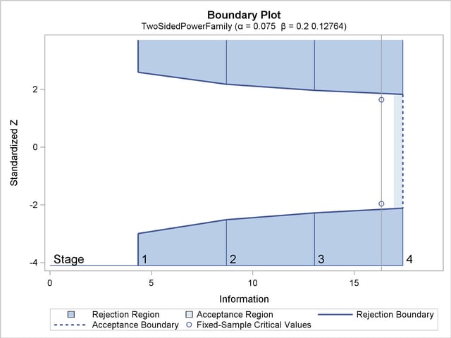
The "Boundary Information" table in Output 78.7.2 displays the information level, alternative reference, and boundary values at each stage. With the default BOUNDARYSCALE=STDZ option, the procedure displays the output boundaries with the standardized  statistic.
| Boundary Information (Standardized Z Scale) Null Reference = 0 |
|||||||
|---|---|---|---|---|---|---|---|
| _Stage_ | Alternative | Boundary Values | |||||
| Information Level | Reference | Lower | Upper | ||||
| Proportion | Actual | Events | Lower | Upper | Alpha | Alpha | |
| 1 | 0.2500 | 4.348221 | 19.32543 | -1.44538 | 1.44538 | -2.98871 | 2.59149 |
| 2 | 0.5000 | 8.696441 | 38.65085 | -2.04408 | 2.04408 | -2.51320 | 2.17917 |
| 3 | 0.7500 | 13.04466 | 57.97628 | -2.50348 | 2.50348 | -2.27093 | 1.96910 |
| 4 | 1.0000 | 17.39288 | 77.3017 | -2.89077 | 2.89077 | -2.11334 | 1.83246 |
With the specified ODS GRAPHICS ON statement, a detailed boundary plot with the rejection and acceptance regions is displayed, as shown in Output 78.7.3.
With the MODEL=PHREG option in the SAMPLESIZE statement, the "Sample Size Summary" table in Output 78.7.4 displays the parameters used in the sample size computation for the proportional hazards regression model.
With a minimum accrual time of  weeks and maximum accrual time of
  weeks, an accrual time of
  weeks is used in the study. The "Numbers of Events" table in Output 78.7.5 displays the required numbers of events for the group sequential clinical trial.
The following statements invoke the SEQDESIGN procedure and provide more detailed sample size information with a -week accrual time:
   proc seqdesign altref=0.69315;
      TwoSidedPowerFamily: design method=pow
                                  nstages=4
                                  alpha=0.075(lower=0.025)
                                  beta=0.20;
      samplesize model=phreg( xvariance=0.25 xrsquare=0.10
                              hazard=0.02451
                              accrate=10 acctime=20);
   ods output Boundary=Bnd_Time;
   run;
The ODS OUTPUT statement with the BOUNDARY=BND_TIME option creates an output data set named BND_TIME which contains the resulting boundary information for the subsequent sequential tests.
With an accrual time of weeks, the "Sample Size Summary" table in Output 78.7.6 displays the follow-up time for the trial.
| Sample Size Summary | |
|---|---|
| Test | PH Reg Parameter |
| Parameter | 0.69315 |
| X Variance | 0.25 |
| R Square (X) | 0.1 |
| Hazard Rate | 0.02451 |
| Accrual Rate | 10 |
| Accrual Time | 20 |
| Follow-up Time | 10.34195 |
| Total Time | 30.34195 |
| Max Number of Events | 77.3017 |
| Max Sample Size | 200 |
| Expected Sample Size (Null Ref) | 199.4282 |
| Expected Sample Size (Alt Ref) | 188.6561 |
The "Numbers of Events and Sample Sizes" table in Output 78.7.7 displays the required sample sizes for the group sequential clinical trial.
| Numbers of Events (D) and Sample Sizes (N) Z Test for PH Regression Parameter |
||||||||
|---|---|---|---|---|---|---|---|---|
| _Stage_ | Fractional Time | Ceiling Time | ||||||
| D | Time | N | Information | D | Time | N | Information | |
| 1 | 19.33 | 13.2362 | 132.36 | 4.3482 | 21.49 | 14 | 140.00 | 4.8359 |
| 2 | 38.65 | 19.1466 | 191.47 | 8.6964 | 41.90 | 20 | 200.00 | 9.4281 |
| 3 | 57.98 | 24.3744 | 200.00 | 13.0447 | 60.14 | 25 | 200.00 | 13.5309 |
| 4 | 77.30 | 30.3420 | 200.00 | 17.3929 | 79.26 | 31 | 200.00 | 17.8346 |
Thus, the study will perform three interim analyses after  , , and
  weeks and a final analysis after
  weeks if the study does not stop at any of the interim analyses.
Suppose  mice are available for the first interim analysis after week . Output 78.7.8 lists the first 10 observations in the data set weeks_1.
The TrtGp variable is a grouping variable with the value for a mouse in the placebo control group and the value for a mouse in the treatment group.
The Weeks variable is the survival time variable measured in weeks and the Event variable is the censoring variable with the value indicating censoring. That is, the values of Weeks are considered censored if the corresponding values of Event are 0; otherwise, they are considered as event times.
The following statements use the PHREG procedure to estimate the treatment effect after adjusting for the Wgt variable at stage :
   proc phreg data=Time_1;
      model Weeks*Event(0)= TrtGp Wgt;
   ods output parameterestimates=Parms_Time1;
   run;
The following statements create and display (in Output 78.7.9) the data set for the treatment effect MLE statistic and its associated standard error. Note that for a MLE statistic, the inverse of the variance of the statistic is the information.
   data Parms_Time1;
      set Parms_Time1;
      if Parameter='TrtGp';
      _Scale_='MLE';
      _Stage_= 1;
      keep _Scale_ _Stage_ Parameter Estimate StdErr;
   run;

   proc print data=Parms_Time1;
      title 'Statistics Computed at Stage 1';
   run;
The following statements invoke the SEQTEST procedure to test for early stopping at stage :
   ods graphics on;
   proc seqtest Boundary=Bnd_Time
                Parms(Testvar=TrtGp)=Parms_Time1
                order=lr
                ;
   ods output Test=Test_Time1;
   run;
   ods graphics off;
The BOUNDARY= option specifies the input data set that provides the boundary information for the trial at stage , which was generated in the SEQDESIGN procedure. The PARMS=PARMS_TIME1 option specifies the input data set PARMS_TIME1 that contains the test statistic and its associated standard error at stage , and the TESTVAR=TRTGP option identifies the test variable TRTGP in the data set.
The ORDER=LR option uses the LR ordering to derive the  -value, the unbiased median estimate, and the confidence limits for the regression slope estimate.
The ODS OUTPUT statement with the TEST=TEST_TIME1 option creates an output data set named TEST_TIME1 which contains the updated boundary information for the test at stage . The data set also provides the boundary information that is needed for the group sequential test at the next stage.
The "Design Information" table in Output 78.7.10 displays design specifications. By default, when the boundary values are modified for the new information levels, the Type I level is maintained. The maximum information and the power have been modified for the new information levels.
| Design Information | |
|---|---|
| BOUNDARY Data Set | WORK.BND_TIME |
| Data Set | WORK.PARMS_TIME1 |
| Statistic Distribution | Normal |
| Boundary Scale | Standardized Z |
| Alternative Hypothesis | Two-Sided |
| Early Stop | Reject Null |
| Number of Stages | 4 |
| Alpha | 0.075 |
| Alpha (Lower) | 0.025 |
| Alpha (Upper) | 0.05 |
| Beta (Lower) | 0.20048 |
| Beta (Upper) | 0.12795 |
| Power (Lower) | 0.79952 |
| Power (Upper) | 0.87205 |
| Max Information (Percent of Fixed Sample) | 106.5982 |
| Max Information | 17.3928828 |
| Null Ref ASN (Percent of Fixed Sample) | 104.4715 |
| Lower Alt Ref ASN (Percent of Fixed Sample) | 79.7886 |
| Upper Alt Ref ASN (Percent of Fixed Sample) | 71.53877 |
The "Test Information" table in Output 78.7.11 displays the boundary values for the test statistic with the MLE statistic scale.
| Test Information (Standardized Z Scale) Null Reference = 0 |
||||||||
|---|---|---|---|---|---|---|---|---|
| _Stage_ | Alternative | Boundary Values | Test | |||||
| Information Level | Reference | Lower | Upper | TrtGp | ||||
| Proportion | Actual | Lower | Upper | Alpha | Alpha | Estimate | Action | |
| 1 | 0.2649 | 4.607347 | -1.48783 | 1.48783 | -2.92457 | 2.54086 | 0.01795 | Continue |
| 2 | 0.5099 | 8.869192 | -2.06428 | 2.06428 | -2.50505 | 2.17290 | . | |
| 3 | 0.7550 | 13.13104 | -2.51175 | 2.51175 | -2.27093 | 1.96941 | . | |
| 4 | 1.0000 | 17.39288 | -2.89077 | 2.89077 | -2.11635 | 1.83531 | . | |
Since only the information level at stage is derived in the PARMS= data set, the information levels at subsequent stages are derived proportionally from the corresponding information levels in the original design. At stage , the standardized statistic  is between the lower and upper boundary values of
  and
and  , so the trial continues to the next stage.
Note that the observed information level  corresponds to a proportion of
  in the information level. If the observed information level is much smaller than the target proportion of
  , then you need to increase the accrual rate, accrual time, or follow-up time to achieve target information levels for subsequent stages. These modifications should be specified in the study plan before the study begins.
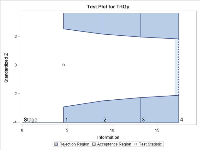
With the specified ODS GRAPHICS ON statement, a boundary plot with test statistics is displayed by default, as shown in Output 78.7.12. As expected, the test statistic is in the continuation region between the lower and upper boundary values.
The following statements use the PHREG procedure to compute the MLE statistic and its associated standard error at stage  :
:
   proc phreg data=Time_2;
      model Weeks*Event(0)= TrtGp Wgt;
   ods output parameterestimates= Parms_Time2;
   run;
The following statements create the data set for the MLE statistic and its associated standard error at stage :
   data Parms_Time2;
      set Parms_Time2;
      if Parameter='TrtGp';
      _Scale_='MLE';
      _Stage_= 2;
      keep _Scale_ _Stage_ Parameter Estimate StdErr;
   run;
The following statements invoke the SEQTEST procedure to test for early stopping at stage :
   proc seqtest Boundary=Test_Time1
                Parms(Testvar=TrtGp)=Parms_Time2
                order=lr
                ;
   ods output Test=Test_Time2;
   run;
The BOUNDARY= option specifies the input data set that provides the boundary information for the trial at stage , which was generated by the SEQTEST procedure at the previous stage. The PARMS= option specifies the input data set that contains the test statistic and its associated standard error at stage , and the TESTVAR= option identifies the test variable in the data set.
The ODS OUTPUT statement with the TEST=TEST_TIME2 option creates an output data set named TEST_TIME2 which contains the updated boundary information for the test at stage . The data set also provides the boundary information that is needed for the group sequential test at the next stage.
The "Test Information" table in Output 78.7.13 displays the boundary values for the test statistic with the MLE statistic scale. At stage , the standardized statistic  is between the lower and upper boundary values,
  and
and  , respectively, so the trial continues to the next stage.
| Test Information (Standardized Z Scale) Null Reference = 0 |
||||||||
|---|---|---|---|---|---|---|---|---|
| _Stage_ | Alternative | Boundary Values | Test | |||||
| Information Level | Reference | Lower | Upper | TrtGp | ||||
| Proportion | Actual | Lower | Upper | Alpha | Alpha | Estimate | Action | |
| 1 | 0.2649 | 4.607347 | -1.48783 | 1.48783 | -2.92457 | 2.54086 | 0.01795 | Continue |
| 2 | 0.5251 | 9.132918 | -2.09475 | 2.09475 | -2.47689 | 2.14819 | -0.43552 | Continue |
| 3 | 0.7625 | 13.2629 | -2.52433 | 2.52433 | -2.26878 | 1.96770 | . | |
| 4 | 1.0000 | 17.39288 | -2.89077 | 2.89077 | -2.12017 | 1.83880 | . | |
Since the data set PARMS_Time2 contains the test information only at stage , the information level at stage in the TEST_Time1 data set is used to generate boundary values for the test.
Similarly, the test statistic at stage  is also between its corresponding lower and upper boundary values. The trial continues to the next stage.
The following statements use the PHREG procedure to compute the MLE statistic and its associated standard error at the final stage:
   proc phreg data=Time_4;
      model Weeks*Event(0)= TrtGp Wgt;
   ods output parameterestimates= Parms_Time4;
   run;
The following statements create and display (in Output 78.7.14) the data set for the MLE statistic and its associated standard error at each stage of the study:
   data Parms_Time4;
      set Parms_Time4;
      if Parameter='TrtGp';
      _Scale_='MLE';
      _Stage_= 4;
      keep _Scale_ _Stage_ Parameter Estimate StdErr;
   run;

   proc print data=Parms_Time4;
      title 'Statistics Computed at Stage 4';
   run;
The following statements invoke the SEQTEST procedure to test the hypothesis at stage  :
:
   ods graphics on;
   proc seqtest Boundary=Test_Time3
                Parms(Testvar=TrtGp)=Parms_Time4
                order=lr
                ;
   run;
   ods graphics off;
The BOUNDARY= option specifies the input data set that provides the boundary information for the trial at stage , which was generated by the SEQTEST procedure at the previous stage. The PARMS= option specifies the input data set that contains the test statistic and its associated standard error at stage , and the TESTVAR= option identifies the test variable in the data set.
The "Test Information" table in Output 78.7.15 displays the boundary values for the test statistic. The standardized test statistic  is between the lower and upper boundary values of
  and
and  , respectively, so the study stops and accepts the null hypothesis. That is, there is no evidence of reduction in hazard rate for the new treatment.
| Test Information (Standardized Z Scale) Null Reference = 0 |
||||||||
|---|---|---|---|---|---|---|---|---|
| _Stage_ | Alternative | Boundary Values | Test | |||||
| Information Level | Reference | Lower | Upper | TrtGp | ||||
| Proportion | Actual | Lower | Upper | Alpha | Alpha | Estimate | Action | |
| 1 | 0.2647 | 4.607347 | -1.48783 | 1.48783 | -2.92457 | 2.54086 | 0.01795 | Continue |
| 2 | 0.5248 | 9.132918 | -2.09475 | 2.09475 | -2.47689 | 2.14819 | -0.43552 | Continue |
| 3 | 0.7095 | 12.34753 | -2.43566 | 2.43566 | -2.32705 | 2.02634 | 0.34864 | Continue |
| 4 | 1.0000 | 17.40274 | -2.89159 | 2.89159 | -2.10447 | 1.82112 | -0.18570 | Accept Null |
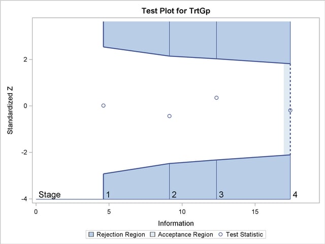
The "Test Plot" displays boundary values of the design and the test statistic at the first two stages, as shown in Output 78.7.16. It also shows that the test statistic is in the "Acceptance Region" between the lower and upper boundary values at stage .
After the stopping of a trial, the "Parameter Estimates" table in Output 78.7.17 displays the stopping stage, parameter estimate, unbiased median estimate, confidence limits, and -value under the null hypothesis  .
.
As expected, the two-sided -value  is not significant at the lower
  level and the upper
  level, and the two-sided
  confidence interval contains the null value zero. The -value, unbiased median estimate, and lower confidence limit depend on the ordering of the sample space
  , where
  is the stage number and
  is the standardized statistic. With the specified LR ordering, the two-sided -value is derived from the one-sided -value
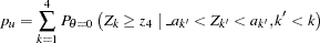 |
where  is the observed test statistic at stage ,
  is a standardized normal variate at stage , and
  and
and  are the stage lower and upper rejection boundary values, respectively.
Thus,
 |
where  is the upper level and
  .
.
Since  ,
,  , which is greater than
  . Thus, the two-sided -value is given by
  .
.
Copyright © 2009 by SAS Institute Inc., Cary, NC, USA. All rights reserved.