| The SEQTEST Procedure |
Example 78.6 Comparing Two Survival Distributions with a Log-Rank Test
This example requests a log-rank test that compares two survival distributions for the treatment effect (Jennison and Turnbull 2000, pp. 77–79; Whitehead 1997, pp. 36–39).
A clinic is studying the effect of a new cancer treatment. The study consists of mice exposed to a carcinogen and randomized to either the control group or the treatment group. The event of interest is the death from cancer induced by the carcinogen, and the response is the time from randomization to death.
Following the derivations in the section "Test for Two Survival Distributions with a Log-Rank Test" in the chapter "The SEQDESIGN Procedure," the hypothesis  with an alternative hypothesis
  can be used, where
  is the hazard ratio between the treatment group and control group.
Suppose that from past experience, the median survival time for the control group is  weeks, and the study would like to detect a
  weeks median survival time with a
  power in the trial. Assuming exponential survival functions for the two groups, the hazard rates can be computed from
 |
where  .
.
Thus, with  and
and  , the hazard ratio
  and the alternative hypothesis is
 |
The following statements invoke the SEQDESIGN procedure and request a four-stage group sequential design for normally distributed data. The design uses a one-sided alternative hypothesis with early stopping to reject and to accept the null hypothesis  . Whitehead’s triangular method is used to derive the boundaries.
   ods graphics on;
   proc seqdesign altref=0.69315
                  boundaryscale=score
                  ;
      OneSidedWhitehead: design method=whitehead
                                nstages=4
                                boundarykey=alpha
                                alt=upper  stop=both
                                beta=0.20;
      samplesize model=twosamplesurvival
                       ( nullhazard=0.03466
                         accrate=10);
   run;
   ods graphics off;
A Whitehead method creates boundaries that approximately satisfy the Type I and Type II error probability level specification. The BOUNDARYKEY=ALPHA option is used to adjust the boundary value at the last stage and to meet the specified Type I probability level.
The specified ACCRATE=10 option indicates that  mice will be accrued each week and the resulting minimum and maximum accrual times are displayed. With the BOUNDARYSCALE=SCORE option, the procedure displays the output boundaries with the score statistics.
The "Design Information" table in Output 78.6.1 displays design specifications and derived statistics.
| Design Information | |
|---|---|
| Statistic Distribution | Normal |
| Boundary Scale | Score |
| Alternative Hypothesis | Upper |
| Early Stop | Accept/Reject Null |
| Method | Whitehead |
| Boundary Key | Alpha |
| Alternative Reference | 0.69315 |
| Number of Stages | 4 |
| Alpha | 0.05 |
| Beta | 0.20044 |
| Power | 0.79956 |
| Max Information (Percent of Fixed Sample) | 129.9894 |
| Max Information | 16.70624 |
| Null Ref ASN (Percent of Fixed Sample) | 62.6302 |
| Alt Ref ASN (Percent of Fixed Sample) | 74.00064 |
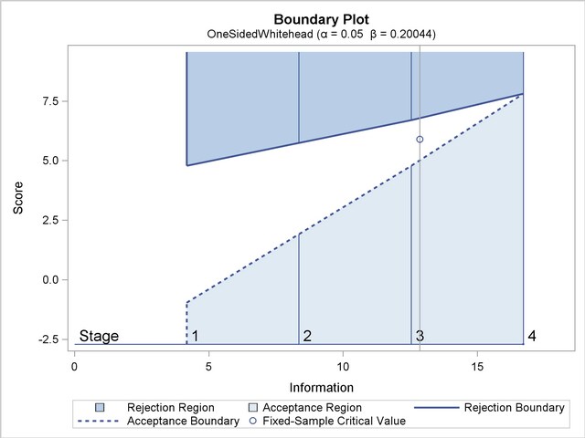
The "Boundary Information" table in Output 78.6.2 displays the information level, alternative reference, and boundary values at each stage.
| Boundary Information (Score Scale) Null Reference = 0 |
||||||
|---|---|---|---|---|---|---|
| _Stage_ | Alternative | Boundary Values | ||||
| Information Level | Reference | Upper | ||||
| Proportion | Actual | Events | Upper | Beta | Alpha | |
| 1 | 0.2500 | 4.176561 | 16.70624 | 2.89498 | -0.95755 | 4.78773 |
| 2 | 0.5000 | 8.353122 | 33.41249 | 5.78997 | 1.91509 | 5.74527 |
| 3 | 0.7500 | 12.52968 | 50.11873 | 8.68495 | 4.78773 | 6.70282 |
| 4 | 1.0000 | 16.70624 | 66.82498 | 11.57993 | 7.81296 | 7.81296 |
With the specified ODS GRAPHICS ON statement, a detailed boundary plot with the rejection and acceptance regions is displayed by default, as shown in Output 78.6.3.
With the MODEL=TWOSAMPLESURVIVAL option in the SAMPLESIZE statement, the "Sample Size Summary" table in Output 78.6.4 displays the parameters for the sample size computation.
| Sample Size Summary | |
|---|---|
| Test | Two-Sample Survival |
| Null Hazard Rate | 0.03466 |
| Hazard Rate (Group A) | 0.01733 |
| Hazard Rate (Group B) | 0.03466 |
| Hazard Ratio | 0.499999 |
| log(Hazard Ratio) | -0.69315 |
| Reference Hazards | Alt Ref |
| Accrual Rate | 10 |
| Min Accrual Time | 6.682498 |
| Min Sample Size | 66.82498 |
| Max Accrual Time | 25.401 |
| Max Sample Size | 254.01 |
| Max Number of Events | 66.82498 |
With a minimum accrual time of  weeks and a maximum accrual time of
  weeks, an accrual time of
  weeks is used in the study.
The "Numbers of Events" table in Output 78.6.5 displays the required number of events for the group sequential clinical trial.
The following statements invoke the SEQDESIGN procedure and provide more detailed sample size information:
   proc seqdesign altref=0.69315
                  boundaryscale=score
                  ;
      OneSidedWhitehead: design method=whitehead
                                nstages=4
                                boundarykey=alpha
                                alt=upper
                                stop=both
                                beta=0.20;
      samplesize model=twosamplesurvival
                       ( nullhazard=0.03466
                         accrate=10 acctime=20);
   ods output Boundary=Bnd_Surv;
   run;
The ODS OUTPUT statement with the BOUNDARY=BND_SURV option creates an output data set named BND_SURV which contains the resulting boundary information for the subsequent sequential tests.
With an accrual time of weeks, the "Sample Size Summary" table in Output 78.6.6 displays the follow-up time for the trial.
| Sample Size Summary | |
|---|---|
| Test | Two-Sample Survival |
| Null Hazard Rate | 0.03466 |
| Hazard Rate (Group A) | 0.01733 |
| Hazard Rate (Group B) | 0.03466 |
| Hazard Ratio | 0.499999 |
| log(Hazard Ratio) | -0.69315 |
| Reference Hazards | Alt Ref |
| Accrual Rate | 10 |
| Accrual Time | 20 |
| Follow-up Time | 6.47422 |
| Total Time | 26.47422 |
| Max Number of Events | 66.82498 |
| Max Sample Size | 200 |
| Expected Sample Size (Null Ref) | 161.5937 |
| Expected Sample Size (Alt Ref) | 172.4689 |
The "Numbers of Events and Sample Sizes" table in Output 78.6.7 displays the required sample sizes for the group sequential clinical trial.
| Numbers of Events (D) and Sample Sizes (N) Two-Sample Log-Rank Test |
||||||||||||||||
|---|---|---|---|---|---|---|---|---|---|---|---|---|---|---|---|---|
| _Stage_ | Fractional Time | Ceiling Time | ||||||||||||||
| D | D(Grp 1) | D(Grp 2) | Time | N | N(Grp 1) | N(Grp 2) | Information | D | D(Grp 1) | D(Grp 2) | Time | N | N(Grp 1) | N(Grp 2) | Information | |
| 1 | 16.71 | 5.82 | 10.89 | 11.9866 | 119.87 | 59.93 | 59.93 | 4.1766 | 16.74 | 5.83 | 10.91 | 12 | 120.00 | 60.00 | 60.00 | 4.1854 |
| 2 | 33.41 | 11.84 | 21.57 | 17.3584 | 173.58 | 86.79 | 86.79 | 8.3531 | 35.73 | 12.68 | 23.04 | 18 | 180.00 | 90.00 | 90.00 | 8.9322 |
| 3 | 50.12 | 18.01 | 32.11 | 21.7479 | 200.00 | 100.00 | 100.00 | 12.5297 | 51.07 | 18.37 | 32.70 | 22 | 200.00 | 100.00 | 100.00 | 12.7667 |
| 4 | 66.82 | 24.46 | 42.37 | 26.4742 | 200.00 | 100.00 | 100.00 | 16.7062 | 68.55 | 25.14 | 43.41 | 27 | 200.00 | 100.00 | 100.00 | 17.1377 |
Thus the study will perform three interim analyses after  ,
,  , and
, and  weeks and a final analysis after
  weeks if the study does not stop at any of the interim analyses.
Note that the SEQDESIGN procedure does not compute numbers of events or sample sizes for all statistical models. If the number of events or sample size for a fixed-sample design is available, then the MODEL=INPUTNEVENTS or MODEL=INPUTNOBS option can be used to input fixed-sample information. For example, with a required fixed-sample number of events  , the following SAMPLESIZE statement can be used to produce the same sample size results:
      samplesize model=inputnevents
                       ( d=51.47 sample=two
                         hazard=0.03466 0.01733
                         accrate=10 acctime=20);
Suppose that  mice are available after week for the first interim analysis. Output 78.6.8 lists the 10 observations in the data set weeks_1.
The TrtGp variable is a grouping variable with the value  for a mouse in the placebo control group and the value
  for a mouse in the treatment group. The Weeks variable is the survival time variable measured in weeks and the Event variable is the censoring variable with the value indicating censoring. That is, the values of Weeks are considered censored if the corresponding values of Event are 0; otherwise, they are considered as event times.
The following statements use the LIFETEST procedure to estimate the log-rank statistic at stage :
   proc lifetest data=Surv_1;
      time Weeks*Event(0);
      test TrtGp;
   ods output logunichisq=Parms_Surv1;
   run;
The following statements create and display (in Output 78.6.9) the data set for the log-rank statistic and its associated standard error:
   data Parms_Surv1;
      set Parms_Surv1(rename=(Statistic=Estimate));
      if Variable='TrtGp';
      _Scale_='Score';
      _Stage_= 1;
      keep Variable _Scale_ _Stage_ StdErr Estimate;
   run;

   proc print data=Parms_Surv1;
      title 'Statistics Computed at Stage 1';
   run;
The following statements invoke the SEQTEST procedure to test for early stopping at stage :
   ods graphics on;
   proc seqtest Boundary=Bnd_Surv
                Parms(Testvar=TrtGp)=Parms_Surv1
                boundaryscale=score
                ;
   ods output Test=Test_Surv1;
   run;
   ods graphics off;
The BOUNDARY= option specifies the input data set that provides the boundary information for the trial at stage , which was generated in the SEQDESIGN procedure. The PARMS=PARMS_SURV1 option specifies the input data set PARMS_SURV1 that contains the test statistic and its associated standard error at stage , and the TESTVAR=TRTGP option identifies the test variable TRTGP in the data set.
The ODS OUTPUT statement with the TEST=TEST_SURV1 option creates an output data set named TEST_SURV1 which contains the updated boundary information for the test at stage . The data set also provides the boundary information that is needed for the group sequential test at the next stage.
The "Design Information" table in Output 78.6.10 displays design specifications. By default, when the boundary values are modified for the new information levels, the Type I  level is maintained. The maximum information and the power have been modified for the new information levels.
| Design Information | |
|---|---|
| BOUNDARY Data Set | WORK.BND_SURV |
| Data Set | WORK.PARMS_SURV1 |
| Statistic Distribution | Normal |
| Boundary Scale | Score |
| Alternative Hypothesis | Upper |
| Early Stop | Accept/Reject Null |
| Number of Stages | 4 |
| Alpha | 0.05 |
| Beta | 0.20007 |
| Power | 0.79993 |
| Max Information (Percent of Fixed Sample) | 129.854 |
| Max Information | 16.7062448 |
| Null Ref ASN (Percent of Fixed Sample) | 62.56841 |
| Alt Ref ASN (Percent of Fixed Sample) | 74.05609 |
The "Test Information" table in Output 78.6.11 displays the boundary values for the test statistic with the SCORE statistic scale. Since only the information level at stage is specified in the DATA= data set, the information levels at subsequent stages are derived proportionally from the corresponding information levels in the original design. At stage , the score statistic  is between the upper
  boundary value
  and the upper boundary value
  , so the trial continues to the next stage.
| Test Information (Score Scale) Null Reference = 0 |
|||||||
|---|---|---|---|---|---|---|---|
| _Stage_ | Alternative | Boundary Values | Test | ||||
| Information Level | Reference | Upper | TrtGp | ||||
| Proportion | Actual | Upper | Beta | Alpha | Estimate | Action | |
| 1 | 0.2389 | 3.991698 | 2.76685 | -1.04069 | 4.71422 | 3.20040 | Continue |
| 2 | 0.4926 | 8.22988 | 5.70454 | 1.81950 | 5.72627 | . | |
| 3 | 0.7463 | 12.46806 | 8.64224 | 4.73885 | 6.68621 | . | |
| 4 | 1.0000 | 16.70624 | 11.57993 | 7.80104 | 7.80104 | . | |
Note that the observed information level  corresponds to a proportion of
  in information level. If the observed information level is much smaller than the target proportion of
  , then you need to increase the accrual rate, accrual time, or follow-up time to achieve the target maximum information level for the trial. Scharfstein and Tsiatis (1998) use the simulation and bootstrap methods to modify the trial at interim stages to achieve the target maximum information level. These modifications should be specified in the study protocol or study plan before the study starts.
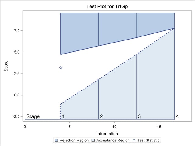
With the specified ODS GRAPHICS ON statement, a boundary plot with test statistics is displayed, as shown in Output 78.6.12. As expected, the test statistic is in the continuation region between the upper and boundary values.
Note that the input DATA= option can also be used for the test statistics. For example, the following statements create and display (in Output 78.6.13) the data set for the log-rank statistic and its associated standard error after the LIFETEST procedure. Since the log-rank statistic is a score statistic, the corresponding information level is the variance of the statistic.
   proc lifetest data=Surv_1;
      time Weeks*Event(0);
      test TrtGp;
   ods output logunichisq=Parms_Surv1a;
   run;
   data Parms_Surv1a;
      set Parms_Surv1a(rename=(Statistic=TrtGp));
      keep _Scale_ _Stage_ _Info_ TrtGp;
      _Scale_='Score';
      _Stage_= 1;
      _Info_= StdErr * StdErr;
      if Variable='TrtGp';
   run;
   proc print data=Parms_Surv1a;
      title 'Statistics Computed at Stage 1';
   run;
The following statements can be used to invoke the SEQTEST procedure to test for early stopping at stage :
   ods graphics on;
   proc seqtest Boundary=Bnd_Surv
                Data(Testvar=TrtGp)=Parms_Surv1a
                boundaryscale=score
                ;
   ods output Test=Test_Surv1;
   run;
   ods graphics off;
The following statements use the LIFETEST procedure to compute the log-rank statistic and its associated standard error at stage  :
:
   proc lifetest data=Surv_2;
      time Weeks*Event(0);
      test TrtGp;
   ods output logunichisq=Parms_Surv2;
   run;
The following statements create and display (in Output 78.6.14) the data set for the log-rank statistic and its associated standard error for each of the first two stages:
   data Parms_Surv2;
      set Parms_Surv2 (rename=(Statistic=Estimate));
      if Variable='TrtGp';
      _Scale_='Score';
      _Stage_= 2;
      keep Variable _Scale_ _Stage_ StdErr Estimate;
   run;

   proc print data=Parms_Surv2;
      title 'Statistics Computed at Stage 2';
   run;
The following statements invoke the SEQTEST procedure to test for early stopping at stage :
   ods graphics on;
   proc seqtest Boundary=Test_Surv1
                Parms(Testvar=TrtGp)=Parms_Surv2
                boundaryscale=score
                citype=lower
                ;
   ods output Test=Test_Surv2;
   run;
   ods graphics off;
The BOUNDARY= option specifies the input data set that provides the boundary information for the trial at stage , which was generated by the SEQTEST procedure at the previous stage. The PARMS= option specifies the input data set that contains the test statistic and its associated standard error at stage , and the TESTVAR= option identifies the test variable in the data set.
The ODS OUTPUT statement with the TEST=TEST_SURV2 option creates an output data set named TEST_SURV2 which contains the updated boundary information for the test at stage . The data set also provides the boundary information that is needed for the group sequential test at the next stage if the trial does not stop at the current stage.
The "Test Information" table in Output 78.6.15 displays the boundary values for the test statistic. The test statistic  is larger than the corresponding upper boundary
  , so the study stops and rejects the null hypothesis. That is, there is evidence of reduction in hazard rate for the new treatment.
| Test Information (Score Scale) Null Reference = 0 |
|||||||
|---|---|---|---|---|---|---|---|
| _Stage_ | Alternative | Boundary Values | Test | ||||
| Information Level | Reference | Upper | TrtGp | ||||
| Proportion | Actual | Upper | Beta | Alpha | Estimate | Action | |
| 1 | 0.2389 | 3.991698 | 2.76685 | -1.04069 | 4.71422 | 3.20040 | Continue |
| 2 | 0.5205 | 8.696125 | 6.02772 | 2.15758 | 5.79895 | 7.31365 | Reject Null |
| 3 | 0.7603 | 12.70118 | 8.80383 | 4.85836 | 6.77006 | . | |
| 4 | 1.0000 | 16.70624 | 11.57993 | 7.79713 | 7.79713 | . | |
With the specified ODS GRAPHICS ON statement, the "Test Plot" displays boundary values of the design and the test statistic at the first two stages, as shown in Output 78.6.16. It also shows that the test statistic is in the "Rejection Region" above the upper boundary value at stage .

After the stopping of a trial, the "Parameter Estimates" table in Output 78.6.17 displays the stopping stage, parameter estimate, unbiased median estimate, confidence limits, and  -value under the null hypothesis
  .
.
As expected, the -value  is significant at the
  level and the lower
  confidence limit is larger than
  . The -value, unbiased median estimate, and lower confidence limit depend on the ordering of the sample space
  , where
  is the stage number and
  is the standardized
  statistic. With the specified stagewise ordering, the -value is
  , where
  is the spending at stage ,
 |
 |
where  is a standardized normal variate and
  is the information level at stage for
  .
.
Copyright © 2009 by SAS Institute Inc., Cary, NC, USA. All rights reserved.