| The NLIN Procedure |
| PROC NLIN Statement |
The PROC NLIN statement invokes the procedure.
The following table lists important options available in the PROC NLIN statement. All options are subsequently discussed in alphabetical order.
Option |
Description |
|---|---|
Options Related to Data Sets |
|
specifies input data set |
|
specifies output data set for parameter estimates, covariance matrix, etc. |
|
requests that final estimates be added to the OUTEST= data set |
|
Optimization Options |
|
limits display of grid search |
|
chooses the optimization method |
|
specifies maximum number of iterations |
|
specifies maximum number of step halvings |
|
allows objective function to increase between iterations |
|
controls the step-size search |
|
specifies the step-size search method |
|
controls the step-size search |
|
uses Moore-Penrose inverse |
|
does not expense degrees of freedom when bounds are active |
|
specifies fixed value for residual variance |
|
Singularity and Convergence Criteria |
|
tunes the convergence criterion |
|
uses the change in loss function as the convergence criterion and tunes its value |
|
uses the maximum change in parameter estimates as the convergence criterion and tunes its value |
|
tunes the singularity criterion used in matrix inversions |
|
Displayed Output |
|
adds Hougaard’s skewness measure to the "Parameter Estimates" table |
|
suppresses the "Iteration History" table |
|
suppresses displayed output |
|
displays model program and variable list |
|
displays the model program code |
|
displays dependencies of model variables |
|
displays the derivative table |
|
adds uncorrected or corrected total sum of squares to the analysis of variance table |
|
displays cross-reference of variables |
|
Trace Model Execution |
|
displays execution messages for program statements |
|
displays results of statements in model program |
|
displays results of operations in model program |
|
-
ALPHA=

specifies the level of significance
used in the construction of  % confidence intervals. The value must be strictly between 0 and 1; the default value of
  results in 95% intervals. This value is used as the default confidence level for limits computed in the "Parameter Estimates" table and with the LCLM, LCL, UCLM, and UCL options in the OUTPUT statement.
 - BEST=n
requests that PROC NLIN display the residual sums of squares only for the best
 combinations of possible starting values from the grid. If you do not specify the BEST= option, PROC NLIN displays the residual sum of squares for every combination of possible parameter starting values.
 - CONVERGE=c
specifies the convergence criterion for PROC NLIN. For all iterative methods the relative offset convergence measure of Bates and Watts is used by default to determine convergence. This measure is labeled "R" in the "Estimation Summary" table. The iterations are said to have converged for CONVERGE=
 if
if 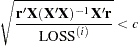
where
 is the residual vector and
  is the
  matrix of first derivatives with respect to the parameters. The default LOSS function is the sum of squared errors (SSE), and
  denotes the value of the loss function at the
  th iteration. By default, CONVERGE=
 . The R convergence measure cannot be computed accurately in the special case of a perfect fit (residuals close to zero). When the SSE is less than the value of the SINGULAR= criterion, convergence is assumed.
 - CONVERGEOBJ=c
uses the change in the LOSS function as the convergence criterion and tunes the criterion. The iterations are said to have converged for CONVERGEOBJ=
if 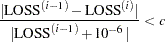
where LOSS
 is the LOSS for the th iteration. The default LOSS function is the sum of squared errors (SSE), the residual sum of squares. The constant should be a small positive number. For more details about the LOSS function, see the section Special Variable Used to Determine Convergence Criteria. For more details about the computational methods in the NIN procedure, see the section Computational Methods.
 Note that in SAS 6 the CONVERGE= and CONVERGEOBJ= options both requested that convergence be tracked by the relative change in the loss function. If you specify the CONVERGEOBJ= option in newer releases, the CONVERGE= option is disabled. This enables you to track convergence as in SAS 6.
- CONVERGEPARM=c
uses the maximum change among parameter estimates as the convergence criterion and tunes the criterion. The iterations are said to have converged for CONVERGEPARM=
if 
where
 is the value of the
  th parameter at the th iteration.
 The default convergence criterion is CONVERGE. If you specify CONVERGEPARM=
, the maximum change in parameters is used as the convergence criterion. If you specify both the CONVERGEOBJ= and CONVERGEPARM= options, PROC NLIN continues to iterate until the decrease in LOSS is sufficiently small (as determined by the CONVERGEOBJ= option) and the maximum change among the parameters is sufficiently small (as determined by the CONVERGEPARM= option). - DATA=SAS-data-set
specifies the input SAS data set to be analyzed by PROC NLIN. If you omit the DATA= option, the most recently created SAS data set is used.
- FLOW
displays a message for each statement in the model program as it is executed. This debugging option is rarely needed, and it produces large amounts of output.
- G4
uses a Moore-Penrose inverse (
 -inverse) in parameter estimation. See Kennedy and Gentle (1980) for details.
 - HOUGAARD
adds Hougaard’s measure of skewness to the "Parameter Estimates" table (Hougaard 1982, 1985). The skewness measure is one method of assessing a parameter estimator’s close-to-linear behavior in the sense of Ratkowsky (1983, 1990). The behavior of estimators that are close to linear approaches that of least-squares estimators in linear models, which are unbiased and have minimum variance. When you specify the HOUGAARD option, the standardized skewness measure of Hougaard (1985) is added for each parameter to the "Parameter Estimates" table. Because of the linkage between nonlinear behavior of a parameter estimator in nonlinear regression and the nonnormality of the estimator’s sampling distribution, Ratkowsky (1990, p. 28) provides the following rules to interpret the (standardized) Hougaard skewness measure:
Values less than 0.1 in absolute value indicate very close-to-linear behavior.
Values between 0.1 and 0.25 in absolute value indicate reasonably close-to-linear behavior.
The nonlinear behavior is apparent for absolute values above 0.25 and is considerable for absolute values above 1.
See the section Hougaard’s Measure of Skewness for further details. Example 60.4 shows how to use this measure to evaluate changes in the parameterization of a nonlinear model. Computation of the Hougaard skewness measure requires first and second derivatives. If you do not provide derivatives with the DER statement—and it is recommended that you do not—the analytic derivatives are computed for you.
- LIST
displays the model program and variable lists, including the statements added by macros. Note that the expressions displayed by the LIST option do not necessarily represent the way the expression is actually calculated—because intermediate results for common subexpressions can be reused—but are shown in expanded form. To see how the expression is actually evaluated, use the LISTCODE option.
- LISTALL
- LISTCODE
displays the derivative tables and the compiled model program code. The LISTCODE option is a debugging feature and is not normally needed.
- LISTDEP
produces a report that lists, for each variable in the model program, the variables that depend on it and the variables on which it depends.
- LISTDER
displays a table of derivatives. The derivatives table lists each nonzero derivative computed for the problem. The derivative listed can be a constant, a variable in the model program, or a special derivative variable created to hold the result of an expression.
- MAXITER=n
specifies the maximum number
of iterations in the optimization process. The default is  .
. - MAXSUBIT=n
places a limit on the number of step halvings. The value of MAXSUBIT must be a positive integer and the default value is
 .
. - METHOD=GAUSS
- METHOD=MARQUARDT
- METHOD=NEWTON
- METHOD=GRADIENT
specifies the iterative method employed by the NLIN procedure in solving the nonlinear least-squares problem. The GAUSS, MARQUARDT, and NEWTON methods are more robust than the GRADIENT method. If you omit the METHOD= option, METHOD=GAUSS is used. See the section Computational Methods for more information.
- NOITPRINT
- NOHALVE
removes the restriction that the objective value must decrease at every iteration. Step halving is still used to satisfy BOUNDS and to ensure that the number of observations that can be evaluated does not decrease. The NOHALVE option can be useful in weighted nonlinear least-squares problems where the weights depend on the parameters, such as in iteratively reweighted least-squares (IRLS) fitting. See Example 60.2 for an application of IRLS fitting.
- NOPRINT
suppresses the display of the output. Note that this option temporarily disables the Output Delivery System (ODS). For more information, see Chapter 20, Using the Output Delivery System.
- OUTEST=SAS-data-set
specifies an output data set that contains the parameter estimates produced at each iteration. See the section Output Data Sets for details. If you want to create a permanent SAS data set, you must specify a two-level name. See the chapter "SAS Files" in SAS Language Reference: Concepts for more information about permanent SAS data sets.
displays the result of each statement in the program as it is executed. This option is a debugging feature that produces large amounts of output and is normally not needed.
- RHO=value
specifies a value that controls the step-size search. By default RHO=0.1, except when METHOD=MARQUARDT. In that case, RHO=10. See the section Step-Size Search for more details.
- SAVE
specifies that, when the iteration limit is exceeded, the parameter estimates from the final iteration be output to the OUTEST= data set. These parameter estimates are associated with the observation for which _TYPE_="FINAL". If you omit the SAVE option, the parameter estimates from the final iteration are not output to the data set unless convergence has been attained.
- SIGSQ=value
specifies a value to use as the estimate of the residual variance in lieu of the estimated mean-squared error. This value is used in computing the standard errors of the estimates. Fixing the value of the residual variance can be useful, for example, in maximum likelihood estimation.
- SINGULAR=s
specifies the singularity criterion,
 , which is the absolute magnitude of the smallest pivot value allowed when inverting the Hessian or the approximation to the Hessian. The default value is
  times the machine epsilon; this product is approximately
  on most computers.
 - SMETHOD=HALVE
- SMETHOD=GOLDEN
- SMETHOD=CUBIC
specifies the step-size search method. The default is SMETHOD=HALVE. See the section Step-Size Search for details.
- TAU=value
specifies a value that is used to control the step-size search. The default is TAU=1, except when METHOD=MARQUARDT. In that case the default is TAU=0.01. See the section Step-Size Search for details.
- TOTALSS
adds to the analysis of variance table the uncorrected total sum of squares in models that have an (implied) intercept, and adds the corrected total sum of squares in models that do not have an (implied) intercept.
- TRACE
displays the result of each operation in each statement in the model program as it is executed, in addition to the information displayed by the FLOW and PRINT options. This debugging option is needed very rarely, and it produces even more output than the FLOW and PRINT options.
- XREF
displays a cross-reference of the variables in the model program showing where each variable is referenced or given a value. The XREF listing does not include derivative variables.
- UNCORRECTEDDF
specifies that no degrees of freedom be lost when a bound is active. When the UNCORRECTEDDF option is not specified, an active bound is treated as if a restriction were applied to the set of parameters, so one parameter degree of freedom is deducted.
Copyright © 2009 by SAS Institute Inc., Cary, NC, USA. All rights reserved.