| The NLIN Procedure |
| Computational Methods |
Nonlinear Least Squares
Recall the basic notation for the nonlinear regression model from the section Notation for Nonlinear Regression Models. The parameter vector  belongs to
  , a subset of
  . Two points of this set are of particular interest: the true value
  and the least-squares estimate
  . The general nonlinear model fit with the NLIN procedure is represented by the equation
 |
where  denotes the
  vector of the
  th regressor (independent) variable, is the true value of the parameter vector, and
  is the vector of homoscedastic and uncorrelated model errors with zero mean.
To write the model for the  th observation, the th elements of
  are collected in the row vector
  , and the model equation becomes
 |
The shorthand  will also be used throughout to denote the mean of the th observation.
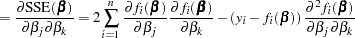
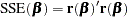
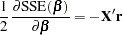
For any given value we can compute the residual sum of squares
 |
 |
|||
 |
 |
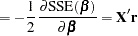
The aim of nonlinear least-squares estimation is to find the value that minimizes  . Because
  is a nonlinear function of , a closed-form solution does not exist for this minimization problem. An iterative process is used instead. The iterative techniques that PROC NLIN uses are similar to a series of linear regressions involving the matrix
  and the residual vector
  , evaluated at the current values of .
It is more insightful, however, to describe the algorithms in terms of their approach to minimizing the residual sum of squares and in terms of their updating formulas. If  denotes the value of the parameter estimates at the
  th iteration, and
  are your starting values, then the NLIN procedure attempts to find values
  and
and  such that
 |
and
 |
The various methods to fit a nonlinear regression model—which you can select with the METHOD= option in the PROC NLIN statement—differ in the calculation of the update vector .
The gradient and Hessian of the residual sum of squares with respect to individual parameters and pairs of parameters are, respectively,
 |
 |
|||
 |
 |
Denote as  the Hessian matrix of the mean function,
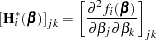 |
Collecting the derivatives across all parameters leads to the expressions
 |
 |
|||
 |
 |
The change in the vector of parameter estimates is computed as follows, depending on the estimation method:
 |
 |
|||
 |
 |
|||
 |
 |
|||
 |
 |
The Gauss-Newton and Marquardt iterative methods regress the residuals onto the partial derivatives of the model with respect to the parameters until the estimates converge. You can view the Marquardt algorithm as a Gauss-Newton algorithm with a ridging penalty. The Newton iterative method regresses the residuals onto a function of the first and second derivatives of the model with respect to the parameters until the estimates converge. Analytical first- and second-order derivatives are automatically computed as needed.
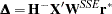
The default method used to compute  is the sweep (Goodnight 1979). It produces a reflexive generalized inverse (a
  -inverse, Pringle and Rayner, 1971). In some cases it might be preferable to use a Moore-Penrose inverse (a
  -inverse) instead. If you specify the G4 option in the PROC NLIN statement, a -inverse is used to calculate on each iteration.
The four algorithms are now described in greater detail.
Algorithmic Details
Gauss-Newton and Newton Methods
From the preceding set of equations you can see that the Marquardt method is a ridged version of the Gauss-Newton method. If the ridge parameter  equals zero, the Marquardt step is identical to the Gauss-Newton step. An important difference between the Newton methods and the Gauss-Newton-type algorithms lies in the use of second derivatives. To motivate this distinctive element between Gauss-Newton and the Newton method, focus first on the objective function in nonlinear least squares. To numerically find the minimum of
 |
you can approach the problem by approximating the sum of squares criterion by a criterion for which you can compute a closed-form solution. Following Seber and Wild (1989, Sect. 2.1.3), we can achieve that by doing the following:
approximating the model and substituting the approximation into
approximating
directly
The first method, approximating the nonlinear model with a first-order Taylor series, is the purview of the Gauss-Newton method. Approximating the residual sum of squares directly is the realm of the Newton method.
The first-order Taylor series of the residual  at the point is
 |
Substitution into leads to the objective function for the Gauss-Newton step:
 |
"Hat" notation is used here to indicate that the quantity in question is evaluated at .
To motivate the Newton method, take a second-order Taylor series of around the value :
 |
Both  and
and  are quadratic functions in and are easily minimized. The minima occur when
 |
 |
|||
 |
 |
and these terms define the preceding update vectors.
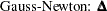
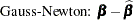
Gauss-Newton Method
Since the Gauss-Newton method is based on an approximation of the model, you can also derive the update vector by first considering the "normal" equations of the nonlinear model
 |
and then substituting the Taylor approximation
 |
for  . This leads to
 |
 |
|||
 |
 |
|||
 |
 |
and the update vector becomes
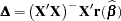 |
Caution:If  is singular or becomes singular, PROC NLIN computes by using a generalized inverse for the iterations after singularity occurs. If is still singular for the last iteration, the solution should be examined.
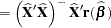
Newton Method
The Newton method uses the second derivatives and solves the equation
 |
If the automatic variables _WEIGHT_, _WGTJPJ_, and _RESID_ are used, then
 |
is the direction, where
 |
and

is an
 diagonal matrix with elements
  of weights from the _WEIGHT_ variable. Each element contains the value of _WEIGHT_ for the th observation.
is an
diagonal matrix with elements  of weights from the _WGTJPJ_ variable.
 Each element
contains the value of _WGTJPJ_ for the th observation. 
is a vector with elements
 from the _RESID_ variable. Each element contains the value of _RESID_ evaluated for the th observation.
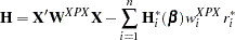
Marquardt Method
The updating formula for the Marquardt method is as follows:
 |
The Marquardt method is a compromise between the Gauss-Newton and steepest descent methods (Marquardt 1963). As  , the direction approaches Gauss-Newton. As
  , the direction approaches steepest descent.
Marquardt’s studies indicate that the average angle between Gauss-Newton and steepest descent directions is about  . A choice of between 0 and infinity produces a compromise direction.
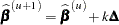
By default, PROC NLIN chooses  to start and computes . If
 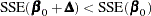 , then
  for the next iteration. Each time
 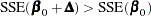 , then
  .
.
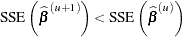
Note:If the SSE decreases on each iteration, then , and you are essentially using the Gauss-Newton method. If SSE does not improve, then is increased until you are moving in the steepest descent direction.
Marquardt’s method is equivalent to performing a series of ridge regressions, and it is useful when the parameter estimates are highly correlated or the objective function is not well approximated by a quadratic.
Steepest Descent (Gradient) Method
The steepest descent method is based directly on the gradient of  :
:
 |
The quantity  is the gradient along which
  increases. Thus
  is the direction of steepest descent.
If the automatic variables _WEIGHT_ and _RESID_ are used, then
 |
is the direction, where
is an
diagonal matrix with elements of weights from the _WEIGHT_ variable. Each element contains the value of _WEIGHT_ for the th observation. is a vector with elements
 from _RESID_. Each element contains the value of _RESID_ evaluated for the th observation.
Using the method of steepest descent, let
 |
where the scalar  is chosen such that
 |
Caution:The steepest-descent method can converge very slowly and is therefore not generally recommended. It is sometimes useful when the initial values are poor.
Step-Size Search
The default method of finding the step size is step halving by using SMETHOD=HALVE. If 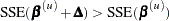 , compute
  ,
,  until a smaller SSE is found.
If you specify SMETHOD=GOLDEN, the step size is determined by a golden section search. The parameter TAU determines the length of the initial interval to be searched, with the interval having length TAU (or  ), depending on
  . The RHO parameter specifies how fine the search is to be. The SSE at each endpoint of the interval is evaluated, and a new subinterval is chosen. The size of the interval is reduced until its length is less than RHO. One pass through the data is required each time the interval is reduced. Hence, if RHO is very small relative to TAU, a large amount of time can be spent determining a step size. For more information about the golden section search, see Kennedy and Gentle (1980).
If you specify SMETHOD=CUBIC, the NLIN procedure performs a cubic interpolation to estimate the step size. If the estimated step size does not result in a decrease in SSE, step halving is used.
Copyright © 2009 by SAS Institute Inc., Cary, NC, USA. All rights reserved.