| The KRIGE2D Procedure |
Example 46.2 Data Quality and Prediction with Missing Values
Kriging methods depend primarily on your data. The quantity and quality of your observations are important factors in minimizing prediction errors and increasing accuracy in your prediction analysis.
A typical aspect of data quality is measurement accuracy. In principle, the accuracy level of your data is not a parameter in kriging prediction; kriging assumes by definition that your data are perfectly accurate (hard) measurements. Whether you accept this assumption depends on your application. For example, an instrumentation error of  1% in the data values might be regarded as considerable in one case, whereas the same level of uncertainty might be trivial within a different framework. Your experience and judgment are crucial when you consider whether observations in a data set might be too noisy for kriging predictions to be useful.
A second aspect of data quality involves the spatial arrangement of your observations. You need to have a sufficient number of observations in order to perform spatial prediction. Also, a key element in minimizing prediction errors is an adequate sampling density. Interpretation of the expressions "sufficient number" and "adequate sampling" is again case-specific. In any event, you want enough measurements so that you can deduce the underlying spatial correlation in the working domain; see also the discussion in the section Choosing the Size of Classes in the VARIOGRAM procedure.
This example focuses on the effects of different sampling densities on the prediction analysis. The demonstration is a slight variation of the example in the section Getting Started: KRIGE2D Procedure. Specifically, you use the same correlation structure and prediction grid. However, the thick data set, is modified as follows: three values in the central area of the grid are assumed missing, namely the observation values at locations  ,
,  , and
, and  . These locations have been selected so that an extended area without observations is created in the domain. The following DATA step is the input for the modified thick data set:
   data thick;
      input East North Thick @@;
      label Thick='Coal Seam Thickness';
      datalines;
       0.7  59.6  34.1   2.1  82.7  42.2   4.7  75.1  39.5
       4.8  52.8  34.3   5.9  67.1  37.0   6.0  35.7  35.9
       6.4  33.7  36.4   7.0  46.7  34.6   8.2  40.1  35.4
      13.3   0.6  44.7  13.3  68.2  37.8  13.4  31.3  37.8
      17.8   6.9  43.9  20.1  66.3  37.7  22.7  87.6  42.8
      23.0  93.9  43.6  24.3  73.0  39.3  24.8  15.1  42.3
      24.8  26.3  39.7  26.4  58.0  36.9  26.9  65.0  37.8
      27.7  83.3  41.8  27.9  90.8  43.3  29.1  47.9  36.7
      29.5  89.4  43.0  30.1   6.1  43.6  30.8  12.1  42.8
      32.7  40.2  37.5  34.8   8.1  43.3  35.3  32.0  38.8
      37.0  70.3  39.2  38.2  77.9  40.7  38.9  23.3  40.5
      39.4  82.5  41.4  43.0   4.7  43.3  43.7   7.6  43.1
      46.4  84.1  41.5  46.7  10.6  42.6  49.9  22.1  40.7
      51.0  88.8  42.0  52.8  68.9     .  52.9  32.7     .
      55.5  92.9  42.2  56.0   1.6  42.7  60.6  75.2  40.1
      62.1  26.6  40.1  63.0  12.7  41.8  69.0  75.6  40.1
      70.5  83.7  40.9  70.9  11.0  41.7  71.5  29.5  39.8
      78.1  45.5  38.7  78.2   9.1  41.7  78.4  20.0  40.8
      80.5  55.9  38.7  81.1  51.0  38.6  83.8   7.9  41.6
      84.5  11.0  41.5  85.2  67.3  39.4  85.5  73.0  39.8
      86.7  70.4  39.6  87.2  55.7  38.8  88.1   0.0  41.6
      88.4  12.1  41.3  88.4  99.6  41.2  88.8  82.9  40.5
      88.9   6.2  41.5  90.6   7.0  41.5  90.7  49.6  38.9
      91.5  55.4  39.0  92.9  46.8  39.1  93.4  70.9  39.7
      55.8  50.5     .  96.2  84.3  40.3  98.2  58.2  39.5
      ;
   title 'Coal Seam Thickness Kriging';
   ods graphics on;
Note that here you assume prior knowledge of the correlation structure model, because its parameters are based on the complete thick data set. A covariance model extracted from the incomplete set with the missing values would be a covariance model coming from a different data set; hence, it is likely to have different parameters.
After you define the modified data set, you run PROC KRIGE2D and request the OBSERVATIONS plot with the SHOWMISSING suboption. You also request two instances of the PREDICTION plot: one that displays the prediction surface and contours, and another that plots the kriging standard error surface and contours. In both of these PREDICTION plots you specify that the observations be shown as gradient markers with outlines. The following statements compute the kriged predictions and produce the requested graphics:
   proc krige2d data=thick outest=predictions
                plots(only)=(observ(showmissing)
                             pred(fill=pred line=pred obs=linegrad)
                             pred(fill=se line=se obs=linegrad));
      coordinates xc=East yc=North;
      predict var=Thick r=60;
      model scale=7.2881 range=30.6239 form=gauss;
      grid x=0 to 100 by 2.5 y=0 to 100 by 2.5;
   run;

   ods graphics off;
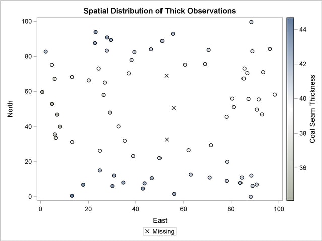
The number of observations table indicates the three missing values in Output 46.2.1.
| Number of Observations Read | 75 |
|---|---|
| Number of Observations Used | 72 |
Output 46.2.2 is a map of the scatter plot of the modified observed data. The SHOWMISSING suboption produces marks in the observations plot that conveniently indicate the locations  ,
,  , and
, and  of the missing values. Consequently, there is now an extended area without any Thick observed values in the central part of the domain.
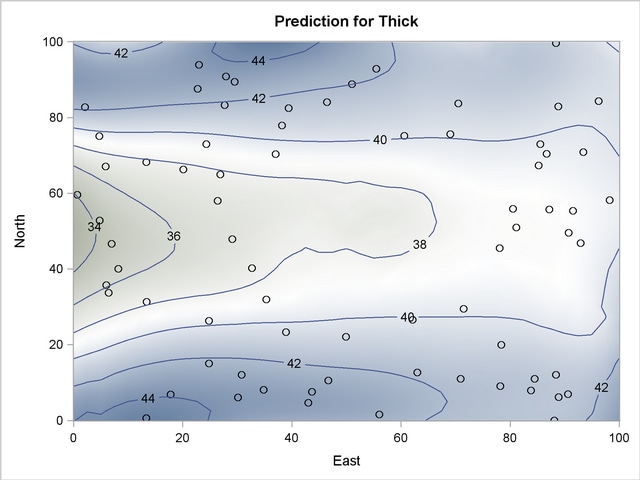
Predictions at grid points with few neighboring data points rely heavily on the underlying covariance structure. The covariance model has a range of about 30,000 feet, which suggests that within this range a grid point might have no data neighbors at all and still obtain a prediction value on the basis of the correlation structure alone. This type of behavior is demonstrated in the Output 46.2.3, which shows a circular region in the center of the plot where there are no data points. Predictions at the nodes in this area are mostly influenced by the covariance structure.
You can see the impact of this effect on the predictions if you compare the prediction contours in the Output 46.2.3 to the ones in Figure 46.4. Despite the contribution of the neighboring Thick data values to the predictions within the area of no observations, the outcome is clearly altered by the absence of observations at the locations , , and .
A noticeable difference is also apparent in the plot of the prediction standard errors. Output 46.2.4 displays these errors, and you can compare it to the standard error surface in Figure 46.4. The comparison shows a slight difference in the color gradient within the area of the missing data values. Output 46.2.4 uses standard error contours to enhance the effect of this difference.
The lack of information from the removed data resulted in an increase of the prediction uncertainty at the grid nodes that are most remotely situated from any observation in the central part of the domain. According to Output 46.2.4, the standard error at these nodes is almost comparable to the error observed near the borders of the domain, where the nodes of the prediction grid have relatively fewer data neighbors than other nodes in the domain.
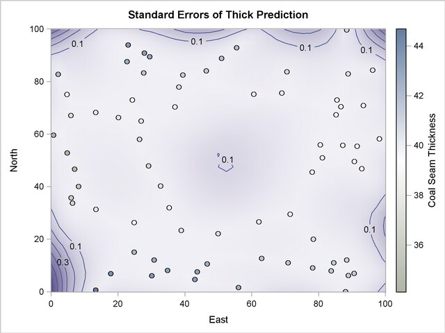
Note that PREDICTION plots display only observations with nonmissing values, as the plots in Output 46.2.3 and Output 46.2.4 demonstrate.
Copyright © 2009 by SAS Institute Inc., Cary, NC, USA. All rights reserved.