| The KRIGE2D Procedure |
| Spatial Prediction Using Kriging, Contour Plots |
After an appropriate semivariogram model is chosen, there are a number of choices involved in producing the kriging surface. In order to illustrate these choices, you use the theoretical semivariogram model that was selected for the coal seam thickness data in Theoretical Semivariogram Model Fitting in the VARIOGRAM procedure. This model is Gaussian,
 |
with a scale of  (that is, the model sill) and a range of
  , based on the weighted least squares fitting results in the PROC VARIOGRAM example.
The first choice is whether to use local or global kriging. Local kriging uses only data points in the neighborhood of a grid point, and you choose this type of analysis by specifying a data search radius around the grid point. Global kriging uses all data points.
The most important consideration in this decision is the spatial covariance structure. Global kriging is appropriate when the correlation range  is approximately equal to the length of the spatial domain. The correlation range is the distance
  (also known as effective or practical range, too) at which the covariance is 5% of its value at zero. That is,
 |
For a Gaussian model, is  52,000 feet. The data points are scattered uniformly throughout a
  (
( ft
ft ) area. Hence, the linear dimension of the data is nearly double the range. This indicates that local kriging rather than global kriging is appropriate because data that are farther away than essentially add to the computational burden without significant contribution to the prediction. The following DATA step is used to input the thickness data set:
   data thick;
      input East North Thick @@;
      label Thick='Coal Seam Thickness';
      datalines;
       0.7  59.6  34.1   2.1  82.7  42.2   4.7  75.1  39.5
       4.8  52.8  34.3   5.9  67.1  37.0   6.0  35.7  35.9
       6.4  33.7  36.4   7.0  46.7  34.6   8.2  40.1  35.4
      13.3   0.6  44.7  13.3  68.2  37.8  13.4  31.3  37.8
      17.8   6.9  43.9  20.1  66.3  37.7  22.7  87.6  42.8
      23.0  93.9  43.6  24.3  73.0  39.3  24.8  15.1  42.3
      24.8  26.3  39.7  26.4  58.0  36.9  26.9  65.0  37.8
      27.7  83.3  41.8  27.9  90.8  43.3  29.1  47.9  36.7
      29.5  89.4  43.0  30.1   6.1  43.6  30.8  12.1  42.8
      32.7  40.2  37.5  34.8   8.1  43.3  35.3  32.0  38.8
      37.0  70.3  39.2  38.2  77.9  40.7  38.9  23.3  40.5
      39.4  82.5  41.4  43.0   4.7  43.3  43.7   7.6  43.1
      46.4  84.1  41.5  46.7  10.6  42.6  49.9  22.1  40.7
      51.0  88.8  42.0  52.8  68.9  39.3  52.9  32.7  39.2
      55.5  92.9  42.2  56.0   1.6  42.7  60.6  75.2  40.1
      62.1  26.6  40.1  63.0  12.7  41.8  69.0  75.6  40.1
      70.5  83.7  40.9  70.9  11.0  41.7  71.5  29.5  39.8
      78.1  45.5  38.7  78.2   9.1  41.7  78.4  20.0  40.8
      80.5  55.9  38.7  81.1  51.0  38.6  83.8   7.9  41.6
      84.5  11.0  41.5  85.2  67.3  39.4  85.5  73.0  39.8
      86.7  70.4  39.6  87.2  55.7  38.8  88.1   0.0  41.6
      88.4  12.1  41.3  88.4  99.6  41.2  88.8  82.9  40.5
      88.9   6.2  41.5  90.6   7.0  41.5  90.7  49.6  38.9
      91.5  55.4  39.0  92.9  46.8  39.1  93.4  70.9  39.7
      55.8  50.5  38.1  96.2  84.3  40.3  98.2  58.2  39.5
      ;
Local kriging is performed by using only data points within a specified radius of each grid point. In this example, a radius of 60,000 feet is used. Other choices involved in local kriging are the minimum and maximum number of data points in each neighborhood (around a grid point). The minimum number is left at the default value of 20; the maximum number defaults to all observations in the data set within the specified radius.
The last step in contouring the data is to define the prediction grid point (node) locations. The prediction grid is typically rectangular, and you decide on the grid points population and spacing based on your available data as well as your application needs. A convenient area that encompasses all the data points is a square of side length 100,000 feet. In the present analysis, a distance of 2,500 feet between nodes in the prediction grid is selected to obtain a smooth contour plot. Based on this choice, you will obtain predictions on a square grid with 41 nodes on each side, which yields a total of 1681 grid points.
You can visualize the outcome of your analysis by using the PLOTS= option in the PROC KRIGE2D statement. PROC KRIGE2D will produce by default one plot that displays the kriging prediction and its corresponding standard error at each output grid point. The locations of the Thick observations are displayed too, as outlines in the default plot. You can also ask for a plot of the thick data set observations and their values by specifying the OBSERV option in the PLOTS option.
The kriging analysis with the KRIGE2D procedure requires that you provide the prediction parameters in the PREDICT statement. You use the VAR= option to specify that you will be using the Thick variable in the kriging system, and the RADIUS= option to specify the radius of the local kriging regression. In this scenario you want to consider for your predictions all the neighboring data within a radius of 60,000 feet from each prediction location. You can specify more than one PREDICT statements; for example, you can do this when you want predictions for different variables in your DATA= data set.
The coordinates of your variable are specified in the COORDINATES statement. The MODEL statement contains the parameters that describe your data spatial correlation. Namely, the FORM= option specifies the model type, based on its mathematical form. The SCALE= and RANGE= options specify the model sill and range, respectively. You can specify more than one MODEL statement for the same PREDICT statement in order to obtain predictions based on different correlation models.
When you use the RADIUS= option to perform local kriging, as in the present example, it is suggested that the radius parameter is at least as large as your model range, so that you do not exclude data points that can contribute to your prediction.
Eventually, you specify the region of predictions with the GRID statement. The following SAS statements compute the kriged surface by using the preceding options and grid choice:
   title 'Coal Seam Thickness Kriging';
   ods graphics on;
   proc krige2d data=thick;
      coordinates xc=East yc=North;
      predict var=Thick radius=60;
      model scale=7.2881 range=30.6239 form=gauss;
      grid x=0 to 100 by 2.5 y=0 to 100 by 2.5;
   run;

   ods graphics off;
The table in Figure 46.1 shows the number of observations read and used in the kriging prediction. This table provides you with useful information in case you have missing values in the input data.
| Number of Observations Read | 75 |
|---|---|
| Number of Observations Used | 75 |
Figure 46.2 shows some general information about the kriging analysis. This includes the count of the output grid points. You have specified the RADIUS= option; therefore you also see that local kriging is requested. Because this is a local analysis, the table also displays the parameters related to the neighborhood search around the grid points.
The covariance model parameters, including the effective range of the Gaussian model you specified, are shown in Figure 46.3.
| Covariance Model Information | |
|---|---|
| Type | Gaussian |
| Sill | 7.2881 |
| Range | 30.6239 |
| Effective Range | 53.042151 |
| Nugget Effect | 0 |
Figure 46.4 shows a map of the kriging prediction contours based on the Thick observations in the specified spatial domain. The prediction error is displayed as a surface in the background.
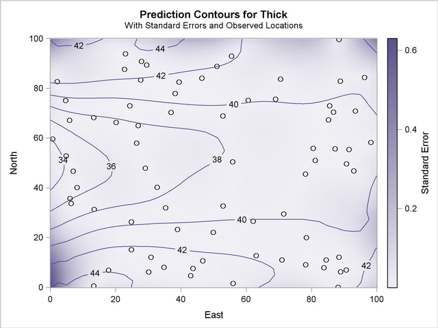
Note the locations of the observed data in Figure 46.4. The figure suggests that the Thick sampling locations are not ideally spread around the prediction area; however, there are no extended areas lacking measurements.
Based on the spatial distribution of the Thick data and the range of your covariance model, you can roughly see that for each prediction location there are at least several neighboring data points that will contribute to the prediction value. Except perhaps for the nodes close to the boundaries of the prediction grid, you can then expect the prediction errors to be reasonably low compared to the predicted Thick values.
The kriging outcome in Figure 46.4 indicates that the standard errors are smaller in the neighborhoods where data are available. The size of these neighborhoods depends on the range of the specified covariance model that characterizes the spatial continuity of the domain, and the prediction radius, if one is specified as in this example. The standard errors tend to increase toward the borders of the prediction area, beyond which no observations are available.
Copyright © 2009 by SAS Institute Inc., Cary, NC, USA. All rights reserved.