| Introduction to Structural Equation Modeling with Latent Variables |
Path Diagrams and the PATH Modeling Language
Complicated models are often easier to understand when they are expressed as path diagrams. One advantage of path diagrams over equations is that variances and covariances can be shown directly in the path diagram. Loehlin (1987) provides a detailed discussion of path diagrams. Another advantage is that the path diagram can be translated easily into the PATH modeling language supported by PROC TCALIS.
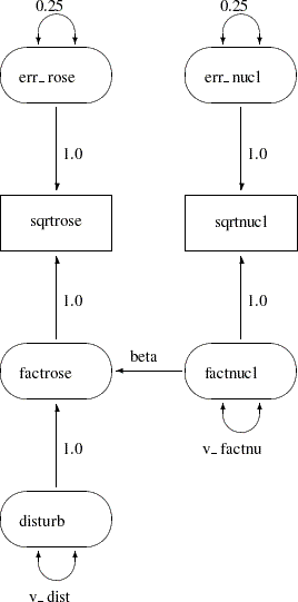
It is customary to write the names of manifest variables in rectangles and the names of latent variables in ovals. The coefficients in each equation are indicated by drawing arrows from the independent variables to the dependent variable. Covariances between exogenous variables are drawn as two-headed arrows. The variance of an exogenous variable can be displayed as a two-headed arrow with both heads pointing to the exogenous variable, since the variance of a variable is the covariance of the variable with itself. Figure 17.5 displays a path diagram for the spleen data, explicitly showing all latent variables (including error terms) and variances of exogenous variables.
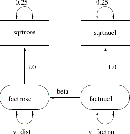
There is an easier way to draw the path diagram based on McArdle’s reticular action model (RAM) (McArdle and McDonald 1984). McArdle uses the convention that a two-headed arrow that points to an endogenous variable actually refers to the error or disturbance term associated with that variable. A two-headed arrow with both heads pointing to the same endogenous variable represents the error or disturbance variance for the equation that determines the endogenous variable; there is no need to draw a separate oval for the error or disturbance term. Similarly, a two-headed arrow connecting two endogenous variables represents the covariance between the error of disturbance terms associated with the endogenous variables. The RAM conventions enable the previous path diagram to be simplified, as shown in Figure 17.6.
The PATH modeling language in PROC TCALIS provides a simple way to transcribe a path diagram based on the reticular action model. In the PATH modeling languages, there are three statements to capture the specifications in path diagrams:
The PATH statement enables you to specify each of the one-headed arrows (paths). The parameters specified in the PATH statement are the path (regression) coefficients.
The PVAR statement enables you to specify each of the double-headed arrows with both heads pointing to the same variable. In general, you specify partial (or total) variance parameters in the PVAR statement. If the variable being pointed at is exogenous, a (total) variance parameter is specified. If the variable being pointed at is endogenous, a partial or an error variance parameter is specified.
The PCOV statement enables you to specify each of the double-headed arrows with its heads pointing to different variables. In general, you specify (partial) covariance parameters in the PCOV statement. The two most common cases are as follows: (1) If the heads of a double-headed arrow are connecting two exogenous variables, a covariance parameter between the two variables is specified; and (2) If the heads of a double-headed arrow are connecting two endogenous variables, an error covariance parameter for the two variables is specified. This error covariance is also a partial covariance between the endogenous variables.
For example, the path diagram for the spleen data in Figure 17.6 can be specified with the PATH modeling language as follows:
   proc tcalis data=spleen outmodel=splmod1;
      path
         sqrtrose <- factrose   1.0,
         sqrtnucl <- factnucl   1.0,
         factrose <- factnucl   beta;
      pvar
         sqrtrose = 0.25,      /* error variance for sqrtrose */
         sqrtnucl = 0.25,      /* error variance for sqrtnucl */
         factrose = v_dist,    /* disturbance variance for factrose */
         factnucl = v_factnu;  /* variance of factnucl */
   run;
One notable item in the specification is that each of the single-headed or double-headed arrows in the path diagram is transcribed into an entry in either the PATH or PVAR statement:
PATH statement:
The paths "sqrtrose <– factrose" and "sqrtnucl <– factnucl" in the PATH statement are followed by the constant 1, indicating fixed path coefficients. The path "factrose <– factnucl" is followed by a parameter named beta, indicating a free path coefficient to estimate in the model.PVAR statement:
A fixed value is specified after the equal signs of sqrtrose and sqrtnucl in the PVAR statement. Because sqrtrose and sqrtnucl are endogenous in the model, you are fixing the error variances of sqrtrose and sqrtnucl to in the specification.
In the last two entries of the PVAR statement, you are putting parameter names after the equal signs. Because factrose and factnucl are exogenous in the model, v_dist and v_factnu are variance parameters of factrose and factnucl, respectively.
Because there are no double-headed arrows each pointing to different variables in the path diagram, the PCOV statement is not needed in the model specification. The resulting output of the PATH model is displayed in Figure 17.7.
In the PROC TCALIS statement, the OUTMODEL=SPLMOD1 option is used. This will save the model specification, together with final estimates in a SAS data set called SPLMOD1. This special type of SAS data set is called "CALISMDL." The following statements are used to display the contents of this OUTMODEL= data set:
   proc print data=splmod1;
   run;
As displayed in Figure 17.8, the first record saves the model type, which is the PATH model specification in this case. The next seven records save the information about the PATH model:  paths and
  partial variances specifications.
| Obs | _TYPE_ | _NAME_ | _VAR1_ | _VAR2_ | _ESTIM_ | _STDERR_ |
|---|---|---|---|---|---|---|
| 1 | MDLTYPE | PATH | . | . | ||
| 2 | LEFT | sqrtrose | factrose | 1.0000 | . | |
| 3 | LEFT | sqrtnucl | factnucl | 1.0000 | . | |
| 4 | LEFT | beta | factrose | factnucl | 0.3907 | 0.07708 |
| 5 | PVAR | sqrtrose | 0.2500 | . | ||
| 6 | PVAR | sqrtnucl | 0.2500 | . | ||
| 7 | PVAR | v_dist | factrose | 0.3815 | 0.28556 | |
| 8 | PVAR | v_factnu | factnucl | 10.5046 | 4.58577 |
In each record, the variables involved, the parameter name, the final estimate, and the standard error estimate are stored. For records with fixed parameters, the parameter names entries are blanks and the standard error estimates are indicated by missing values. This data set can be used as input to another run of the TCALIS procedure with the INMODEL= option in the PROC TCALIS statement. For example, if the iteration limit is exceeded, you can use the CALISMODEL data set to start a new run that begins with the final estimates from the last run. Or you can change the data set to add or remove constraints or modify the model in various other ways. The easiest way to change a CALISMDL data set is to use the FSEDIT procedure, but you can also use a DATA step. For example, you could set the variance of the disturbance term to zero, effectively removing the disturbance from the equation, by removing the parameter name v_dist in the _NAME_ variable and setting the value of the estimate to zero in the _ESTIM_ variable:
   data splmod2(type=calismdl);
      set splmod1;
      if _name_='v_dist' then
         do;
            _name_=' ';
            _estim_=0;
         end;
   run;
Hence, due to the fixed zero error variance for factrose, a model with perfect prediction of factrose from factnucl is specified in the new CALISMDL data set SPLMOD2. This data set serves as the INMODEL= data set in the following statements for another PROC TCALIS run:
   proc tcalis data=spleen inmodel=splmod2;
   run;
The main estimation results are displayed in Figure 17.9.
As can be seen in Figure 17.9, error variance for factrose is a fixed zero in the final results. Because of this modification in the current model specified in the SPLMOD2 data set, the estimates of beta and v_factnu are different from those of the previous model results, which are stored in the SPLMOD1 data set.
Copyright © 2009 by SAS Institute Inc., Cary, NC, USA. All rights reserved.