| The GAM Procedure |
Example 36.2 Poisson Regression Analysis of Component Reliability
In this example, the number of maintenance repairs on a complex system are modeled as realizations of Poisson random variables. The system under investigation has a large number of components, which occasionally break down and are replaced or repaired. During a four-year period, the system was observed to be in a state of steady operation, meaning that the rate of operation remained approximately constant. A monthly maintenance record is available for that period, which tracks the number of components removed for maintenance each month. The data are listed in the following statements, which create a SAS data set:
   title 'Analysis of Component Reliability';
   data equip;
       input year month removals @@;
   datalines;
   1987   1  2 1987   2  4 1987   3  3
   1987   4  3 1987   5  3 1987   6  8
   1987   7  2 1987   8  6 1987   9  3
   1987  10  9 1987  11  4 1987  12 10
   1988   1  4 1988   2  6 1988   3  4
   1988   4  4 1988   5  3 1988   6  5
   1988   7  3 1988   8  4 1988   9  5
   1988  10  3 1988  11  6 1988  12  3
   1989   1  2 1989   2  6 1989   3  1
   1989   4  5 1989   5  5 1989   6  4
   1989   7  2 1989   8  2 1989   9  2
   1989  10  5 1989  11  1 1989  12 10
   1990   1  3 1990   2  8 1990   3 12
   1990   4  7 1990   5  3 1990   6  2
   1990   7  4 1990   8  3 1990   9  0
   1990  10  6 1990  11  6 1990  12  6
   ;
For planning purposes, it is of interest to understand the long- and short-term trends in the maintenance needs of the system. Over the long term, it is suspected that the quality of new components and repair work improves over time, so the number of component removals would tend to decrease from year to year. It is not known whether the robustness of the system is affected by seasonal variations in the operating environment, but this possibility is also of interest.
Because the maintenance record is in the form of counts, the number of removals are modeled as realizations of Poisson random variables. Denote by  the unobserved component removal rate for year
  and month
  . Since the data were recorded at regular intervals (from a system operating at a constant rate), each is assumed to be a function of year and month only.
A preliminary two-way analysis is performed by using PROC GENMOD to make broad inferences on repair trends. A log-link is specified for the model
 |
 |
 |
where  is a grand mean,
  is the effect of the th year, and
  is the effect of the th month. In the following statements, the CLASS statement declares the variables year and month as categorical. Type III sum of squares are requested to test whether there is an overall effect of year and/or month.
   title2 'Two-way model';
   proc genmod data=equip;
       class year month;
       model removals=year month / dist=Poisson link=log type3;
   run;
Output 36.2.1 displays the listed Type III statistics for the fitted model. With the test for year effects yielding a p-value of  , there is no evidence of a long-term trend in maintenance rates. Apparently, the quality of new or repaired components did not change between 1987 and 1990. However, the test for monthly trends does yield a small p-value of
  , indicating that seasonal trends are just barely significant at the
  level.
| LR Statistics For Type 3 Analysis | |||
|---|---|---|---|
| Source | DF | Chi-Square | Pr > ChiSq |
| year | 3 | 2.63 | 0.4527 |
| month | 11 | 21.12 | 0.0321 |
The Type III tests indicate that the year term can be dropped from the model. The focus of the analysis is now on identifying the form of the underlying seasonal trend, which is a task that PROC GAM is especially suited for. PROC GAM will be used to fit both a reduced categorical model, with year eliminated, and a nonparametric spline model. Although PROC GENMOD also has the capability to fit categorical models, as demonstrated earlier, PROC GAM will be used here to fit both models for a better comparison.
The following PROC GAM statements specify the reduced categorical model. For this part of the analysis, a CLASS statement is again used to specify that month is a categorical variable. In the follow-up, the seasonal effect will be treated as a nonparametric function of month.
   title2 'One-way model';
   proc gam data=equip;
        class month;
        model removals=param(month) / dist=Poisson;
        output out=est p;
   run;
The following statements use the SGPLOT procedure to generate a plot of the estimated seasonal trend. The plot is displayed in Output 36.2.2.
   proc sort data=est;by month;run;
   proc sgplot data=est;
       title "Predicted Seasonal Trend";
       yaxis label="Number of Removals";
       xaxis integer values=(1 to 12);
       scatter x=Month y=Removals / name="points"
                                    legendLabel="Removals";
       series  x=Month y=p_Removals / name="line"
                                      legendLabel="Predicted Removals"
                                      lineattrs = GRAPHFIT;
       discretelegend "points" "line";
   run;
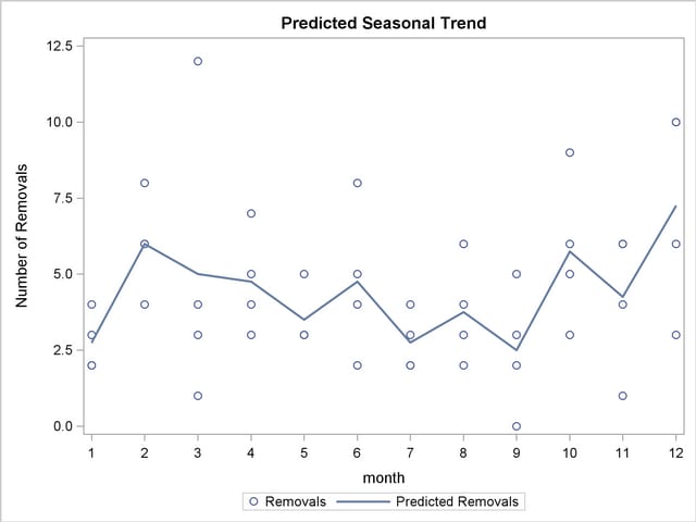
The predicted repair rates shown in Output 36.2.2 form a jagged seasonal pattern. Ignoring the month-to-month fluctuations, which are difficult to explain and can be artifacts of random noise, the general removal rate trend starts by increasing at the beginning of the year; then the trend flattens out in February and then decreases through August; and then it flattens out again in September and begins an increasing trend that continues throughout the rest of the year.
One advantage of nonparametric regression is its ability to highlight general trends in the data, such as those described earlier, and to attribute local fluctuations to unexplained random noise. The nonparametric regression model used by PROC GAM specifies that the underlying removal rates  are of the form
 |
where  is a linear coefficient and
  is a nonparametric regression function. and define the linear and nonparametric parts, respectively, of the seasonal trend.
The following statements request that PROC GAM fit a cubic spline model to the monthly repair data. The output listing is displayed in Output 36.2.3 and Output 36.2.4.
   title 'Analysis of Component Reliability';
   title2 'Spline model';
   proc gam data=equip;
       model removals=spline(month) / dist=Poisson method=gcv;
   run;
The METHOD=GCV option is used to determine an appropriate level of smoothing. The keywords LCLM and UCLM in the OUTPUT statement request that lower and upper 95% confidence bounds on each  be included in the output data set.
| Summary of Input Data Set | |
|---|---|
| Number of Observations | 48 |
| Number of Missing Observations | 0 |
| Distribution | Poisson |
| Link Function | Log |
| Iteration Summary and Fit Statistics | |
|---|---|
| Number of local scoring iterations | 5 |
| Local scoring convergence criterion | 7.241527E-12 |
| Final Number of Backfitting Iterations | 1 |
| Final Backfitting Criterion | 1.710339E-11 |
| The Deviance of the Final Estimate | 56.901543546 |
| Regression Model Analysis Parameter Estimates |
||||
|---|---|---|---|---|
| Parameter | Parameter Estimate |
Standard Error |
t Value | Pr > |t| |
| Intercept | 1.34594 | 0.14509 | 9.28 | <.0001 |
| Linear(month) | 0.02274 | 0.01893 | 1.20 | 0.2362 |
Notice in the listing in Output 36.2.4 that the DF value chosen for the nonlinear portion of the spline by minimizing GCV is about 1.88, which is smaller than the default value of 3. This indicates that the spline model of the seasonal trend is relatively simple. As indicated by the "Analysis of Deviance" table, it is a significant feature of the data: the table lists a p-value of  for the hypothesis of no seasonal trend. Note also that the "Parameter Estimates" table lists a p-value of
  for the hypothesis of no linear factor in the seasonal trend.
The following statements use ODS Graphics statement to plot the smoothing component for the effect of Month on predicted repair rates:
   ods graphics on;

   proc gam data=equip;
       model removals=spline(month) / dist=Poisson method=gcv;
   run;
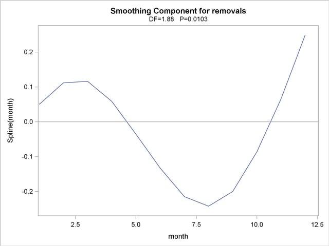
For general information about ODS graphics, see Chapter 21, Statistical Graphics Using ODS. For specific information about the graphics available in the GAM procedure, see the section ODS Graphics. The smoothing component plot is displayed in Output 36.2.5.
In Output 36.2.5, it is apparent that the pattern of repair rates follows the general pattern observed in Output 36.2.2. However, the plot in Output 36.2.5 is much cleaner because the month-to-month fluctuations are smoothed out to reveal the broader seasonal trend.
You can use the PLOTS(CLM) option to added a 95% confidence band to the plot of , as in the following statements:
   proc gam data=equip plots=components(clm);
       model removals=spline(month) / dist=Poisson method=gcv;
   run;

   ods graphics off;
The plot is displayed in Output 36.2.6.
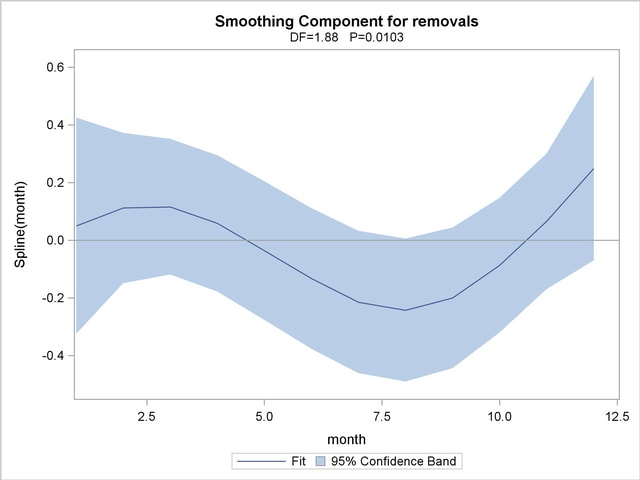
The small p-value in Output 36.2.1 of for the hypothesis of no seasonal trend indicates that the data exhibit significant seasonal structure. However, Output 36.2.6 is a graphical illustration of a degree of indistinctness in that structure. For instance, the horizontal reference line at zero is entirely within the 95% confidence band—that is, the estimated nonlinear part of the trend is relatively flat. Thus, despite evidence of seasonality based on the parametric model, it is difficult to narrow down its significant effects to a specific part of the year.
Copyright © 2009 by SAS Institute Inc., Cary, NC, USA. All rights reserved.