| The GAM Procedure |
Example 36.1 Generalized Additive Model with Binary Data
This example illustrates the capabilities of the GAM procedure and compares it to the GENMOD procedure.
The data used in this example are based on a study by Bell et al. (1994). Bell and his associates studied the result of multiple-level thoracic and lumbar laminectomy, a corrective spinal surgery commonly performed on children. The data in the study consist of retrospective measurements on 83 patients. The specific outcome of interest is the presence (1) or absence (0) of kyphosis, defined as a forward flexion of the spine of at least 40 degrees from vertical. The available predictor variables are age in months at time of the operation (Age), the starting of vertebrae levels involved in the operation (StartVert), and the number of levels involved (NumVert). The goal of this analysis is to identify risk factors for kyphosis. PROC GENMOD can be used to investigate the relationship among kyphosis and the predictors. The following DATA step creates the data kyphosis:
   title 'Comparing PROC GAM with PROC GENMOD';
   data kyphosis;
       input Age StartVert NumVert Kyphosis @@;
   datalines;
   71  5  3  0     158 14 3 0    128 5   4 1
   2   1  5  0     1   15 4 0    1   16  2 0
   61  17 2  0     37  16 3 0    113 16  2 0
   59  12 6  1     82  14 5 1    148 16  3 0
   18  2  5  0     1   12 4 0    243 8   8 0
   168 18 3  0     1   16 3 0    78  15  6 0
   175 13 5  0     80  16 5 0    27  9   4 0
   22  16 2  0     105 5  6 1    96  12  3 1
   131 3  2  0     15  2  7 1    9   13  5 0
   12  2 14  1     8   6  3 0    100 14  3 0
   4   16 3  0     151 16 2 0    31  16  3 0
   125 11 2  0     130 13 5 0    112 16  3 0
   140 11 5  0     93  16 3 0    1   9   3 0
   52  6  5  1     20  9  6 0    91  12  5 1
   73  1  5  1     35  13 3 0    143 3   9 0
   61  1  4  0     97  16 3 0    139 10  3 1
   136 15 4  0     131 13 5 0    121 3   3 1
   177 14 2  0     68  10 5 0    9   17  2 0
   139 6  10 1     2   17 2 0    140 15  4 0
   72  15 5  0     2   13 3 0    120 8   5 1
   51  9  7  0     102 13 3 0    130 1   4 1
   114 8  7  1     81  1  4 0    118 16  3 0
   118 16 4  0     17  10 4 0    195 17  2 0
   159 13 4  0     18  11 4 0    15  16  5 0
   158 15 4  0     127 12 4 0    87  16  4 0
   206 10 4  0     11  15 3 0    178 15  4 0
   157 13 3  1     26  13 7 0    120 13  2 0
   42  6  7  1     36  13 4 0
   ;
   proc genmod data=kyphosis descending;
       model Kyphosis = Age StartVert NumVert/link=logit dist=binomial;
   run;
The GENMOD analysis of the independent variable effects is shown in Output 36.1.1. Based on these results, the only significant factor is StartVert with a log odds ratio of  . The variable NumVert has a p-value of
  with a log odds ratio of
  .
.
| Analysis Of Maximum Likelihood Parameter Estimates | |||||||
|---|---|---|---|---|---|---|---|
| Parameter | DF | Estimate | Standard Error | Wald 95% Confidence Limits | Wald Chi-Square | Pr > ChiSq | |
| Intercept | 1 | -1.2497 | 1.2424 | -3.6848 | 1.1853 | 1.01 | 0.3145 |
| Age | 1 | 0.0061 | 0.0055 | -0.0048 | 0.0170 | 1.21 | 0.2713 |
| StartVert | 1 | -0.1972 | 0.0657 | -0.3260 | -0.0684 | 9.01 | 0.0027 |
| NumVert | 1 | 0.3031 | 0.1790 | -0.0477 | 0.6540 | 2.87 | 0.0904 |
| Scale | 0 | 1.0000 | 0.0000 | 1.0000 | 1.0000 | ||
| Note: | The scale parameter was held fixed. |
The GENMOD procedure assumes a strict linear relationship between the response and the predictors. The following SAS statements use PROC GAM to investigate a less restrictive model, with moderately flexible spline terms for each of the predictors:
   title 'Comparing PROC GAM with PROC GENMOD';
   proc gam data=kyphosis;
      model Kyphosis (event='1') = spline(Age      ,df=3)
                                   spline(StartVert,df=3)
                                   spline(NumVert  ,df=3) / dist=binomial;
   run;
The MODEL statement requests an additive model with a univariate smoothing spline for each term. The response variable option EVENT= chooses Kyphosis (presence) as the event so that the probability of presence of kyphosis is modeled. The option “DIST=BINOMIAL” with binary responses specifies a logistic model. Each term is fit by using a univariate smoothing spline with three degrees of freedom. Of these three degrees of freedom, one is taken up by the linear portion of the fit and two are left for the nonlinear spline portion. Although this might seem to be an unduly modest amount of flexibility, it is better to be conservative with a data set this small.
Output 36.1.2 and Output 36.1.3 list the output from PROC GAM.
| Summary of Input Data Set | |
|---|---|
| Number of Observations | 83 |
| Number of Missing Observations | 0 |
| Distribution | Binomial |
| Link Function | Logit |
| Note: | PROC GAM is modeling the probability that Kyphosis=1. One way to change this to model the probability that Kyphosis=0 is to specify the response variable option EVENT='0'. |
| Iteration Summary and Fit Statistics | |
|---|---|
| Number of local scoring iterations | 9 |
| Local scoring convergence criterion | 2.6635648E-9 |
| Final Number of Backfitting Iterations | 1 |
| Final Backfitting Criterion | 5.2326574E-9 |
| The Deviance of the Final Estimate | 46.610922438 |
| Regression Model Analysis Parameter Estimates |
||||
|---|---|---|---|---|
| Parameter | Parameter Estimate |
Standard Error |
t Value | Pr > |t| |
| Intercept | -2.01533 | 1.45620 | -1.38 | 0.1706 |
| Linear(Age) | 0.01213 | 0.00794 | 1.53 | 0.1308 |
| Linear(StartVert) | -0.18615 | 0.07628 | -2.44 | 0.0171 |
| Linear(NumVert) | 0.38347 | 0.19102 | 2.01 | 0.0484 |
The critical part of the GAM results is the "Analysis of Deviance" table, shown in Output 36.1.3. For each smoothing effect in the model, this table gives a  test comparing the deviance between the full model and the model without this variable. In this case the analysis of deviance results indicates that the effect of Age is highly significant, the effect of StartVert is nearly significant, and the effect of NumVert is insignificant at the 5% level.
PROC GAM can also perform approximate analysis of deviance for smoothing effects by using the ANODEV=NOREFIT option, as in the following statements:
   title 'PROC GAM with Approximate Analysis of Deviance';
   proc gam data=kyphosis;
      model Kyphosis (event='1') = spline(Age      ,df=3)
                                   spline(StartVert,df=3)
                                   spline(NumVert  ,df=3) /
                                       dist=binomial anodev=norefit;
   run;
| Smoothing Model Analysis Approximate Analysis of Deviance |
|||
|---|---|---|---|
| Source | DF | Chi-Square | Pr > ChiSq |
| Spline(Age) | 2.00000 | 7.0888 | 0.0289 |
| Spline(StartVert) | 2.00000 | 5.0431 | 0.0803 |
| Spline(NumVert) | 2.00000 | 2.2471 | 0.3251 |
The "Approximate Analysis of Deviance" table shown in Output 36.1.4 yields similar conclusions to those of the "Analysis of Deviance" table (Output 36.1.3). In addition to the GAM fit that uses all the specified smoothing effects, the default ANODEV=REFIT option requires  additional GAM fits to be performed for smoothing effects. In each of these fits, a submodel is fit by omitting one smoothing term from the model. By contrast, the ANODEV=NOREFIT option keeps the nonparametric terms fixed and requires a weighted least squares fit for only the parametric part of the model. Hence, GAM with the ANODEV=NOREFIT option is computationally inexpensive and is useful for obtaining approximate analysis of deviance results for models with many smoothing effects.
Plots of predictions against predictor can be used to investigate why PROC GAM and PROC GENMOD produce different results. The following statements use ODS Graphics to produce plots of the individual smoothing components. The CLM suboption for the PLOTS option adds a curvewise Bayesian confidence band to each smoothing component, while the COMMONAXES suboption forces all three smoothing component plots to share the same vertical axis limits, allowing a visual judgment of nonparametric effect size.
   ods graphics on;

   proc gam data=kyphosis plots=components(clm commonaxes);
       model Kyphosis (event='1') = spline(Age      ,df=3)
                                    spline(StartVert,df=3)
                                    spline(NumVert  ,df=3) / dist=binomial;
   run;
For general information about ODS Graphics, see Chapter 21, Statistical Graphics Using ODS. For specific information about the graphics available in the GAM procedure, see the section ODS Graphics. The smoothing component plots are displayed in Output 36.1.5.
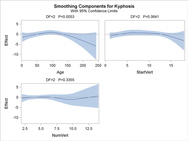
The plots show that the partial predictions corresponding to both Age and StartVert have a quadratic pattern, while NumVert has a more complicated but weaker pattern. However, in the plot for NumVert, notice that about half the vertical range of the function is determined by the point at the upper extreme. It would be a good idea, therefore, to rerun the analysis without this point, to explore how much it affects the conclusions. You can do this by simply including a WHERE clause when specifying the data set for the GAM procedure, as in the following statements:
   proc gam data=kyphosis(where=(NumVert^=14)) plots=components(clm commonaxes);
       model Kyphosis (event='1') = spline(Age      ,df=3)
                                    spline(StartVert,df=3)
                                    spline(NumVert  ,df=3) / dist=binomial;
   run;

   ods graphics off;
The analysis of deviance table from this reanalysis is shown in Output 36.1.6, and Output 36.1.7 shows the recomputed partial predictor plots.
| Smoothing Model Analysis Analysis of Deviance |
||||
|---|---|---|---|---|
| Source | DF | Sum of Squares | Chi-Square | Pr > ChiSq |
| Spline(Age) | 2.00000 | 10.587556 | 10.5876 | 0.0050 |
| Spline(StartVert) | 2.00000 | 5.477094 | 5.4771 | 0.0647 |
| Spline(NumVert) | 2.00000 | 3.209089 | 3.2091 | 0.2010 |
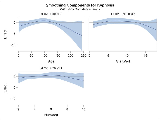
Removing data point NumVert=14 has little effect on either the analysis of deviance results or the estimated curves for StartVert and NumVert. But the removal has a noticeable effect on the variable NumVert, whose curve now also seems quadratic, though it is much less pronounced than for the other two variables.
An important difference between the first analysis of these data with GENMOD and the subsequent analysis with GAM is that GAM indicates that age is a significant predictor of kyphosis. The difference is due to the fact that the GENMOD model includes only a linear effect in Age whereas the GAM model allows a more complex relationship, which the plots indicate is nearly quadratic. Having used the GAM procedure to discover an appropriate form of the dependence of Kyphosis on each of the three independent variables, you can use the GENMOD procedure to fit and assess the corresponding parametric model. The following statements fit a GENMOD model with quadratic terms for all three variables, including tests for the joint linear and quadratic effects of each variable. The resulting contrast tests are shown in Output 36.1.8.
   title 'Comparing PROC GAM with PROC GENMOD';
   proc genmod data=kyphosis(where=(NumVert^=14)) descending;
               model kyphosis = Age       Age      *Age
                                StartVert StartVert*StartVert
                                NumVert   NumVert  *NumVert /
                                    link=logit  dist=binomial;
               contrast 'Age'       Age       1, Age*Age             1;
               contrast 'StartVert' StartVert 1, StartVert*StartVert 1;
               contrast 'NumVert'   NumVert   1, NumVert*NumVert     1;
   run;
| Contrast Results | ||||
|---|---|---|---|---|
| Contrast | DF | Chi-Square | Pr > ChiSq | Type |
| Age | 2 | 13.63 | 0.0011 | LR |
| StartVert | 2 | 15.41 | 0.0005 | LR |
| NumVert | 2 | 3.56 | 0.1684 | LR |
The results for the quadratic GENMOD model are now quite consistent with the GAM results.
From this example, you can see that PROC GAM is very useful in visualizing the data and detecting the nonlinearity among the variables.
Copyright © 2009 by SAS Institute Inc., Cary, NC, USA. All rights reserved.