The CLUSTER Procedure

Getting Started: CLUSTER Procedure

The following example shows how you can use the CLUSTER procedure to compute hierarchical clusters of observations in a SAS data set.

Suppose you want to determine whether national figures for birth rates, death rates, and infant death rates can be used to categorize countries. Previous studies indicate that the clusters computed from this type of data can be elongated and elliptical. Thus, you need to perform a linear transformation on the raw data before the cluster analysis.

The following data¹ from Rouncefield (1995) are birth rates, death rates, and infant death rates for 97 countries. The DATA step creates the SAS data set Poverty:

   data Poverty;
      input Birth Death InfantDeath Country $20. @@;
      datalines;
   24.7  5.7  30.8 Albania             12.5 11.9  14.4 Bulgaria
   13.4 11.7  11.3 Czechoslovakia      12   12.4   7.6 Former_E._Germany
   11.6 13.4  14.8 Hungary             14.3 10.2    16 Poland
   13.6 10.7  26.9 Romania               14    9  20.2 Yugoslavia
   17.7   10    23 USSR                15.2  9.5  13.1 Byelorussia_SSR
   13.4 11.6    13 Ukrainian_SSR       20.7  8.4  25.7 Argentina
   46.6   18   111 Bolivia             28.6  7.9    63 Brazil
   23.4  5.8  17.1 Chile               27.4  6.1    40 Columbia
   32.9  7.4    63 Ecuador             28.3  7.3    56 Guyana
   34.8  6.6    42 Paraguay            32.9  8.3 109.9 Peru
     18  9.6  21.9 Uruguay             27.5  4.4  23.3 Venezuela
     29 23.2    43 Mexico                12 10.6   7.9 Belgium
   13.2 10.1   5.8 Finland             12.4 11.9   7.5 Denmark
   13.6  9.4   7.4 France              11.4 11.2   7.4 Germany
   10.1  9.2    11 Greece              15.1  9.1   7.5 Ireland
    9.7  9.1   8.8 Italy               13.2  8.6   7.1 Netherlands
   14.3 10.7   7.8 Norway              11.9  9.5  13.1 Portugal
   10.7  8.2   8.1 Spain               14.5 11.1   5.6 Sweden
   12.5  9.5   7.1 Switzerland         13.6 11.5   8.4 U.K.
   14.9  7.4     8 Austria              9.9  6.7   4.5 Japan
   14.5  7.3   7.2 Canada              16.7  8.1   9.1 U.S.A.
   40.4 18.7 181.6 Afghanistan         28.4  3.8    16 Bahrain
   42.5 11.5 108.1 Iran                42.6  7.8    69 Iraq
   22.3  6.3   9.7 Israel              38.9  6.4    44 Jordan
   26.8  2.2  15.6 Kuwait              31.7  8.7    48 Lebanon
   45.6  7.8    40 Oman                42.1  7.6    71 Saudi_Arabia
   29.2  8.4    76 Turkey              22.8  3.8    26 United_Arab_Emirates
   42.2 15.5   119 Bangladesh          41.4 16.6   130 Cambodia
   21.2  6.7    32 China               11.7  4.9   6.1 Hong_Kong
   30.5 10.2    91 India               28.6  9.4    75 Indonesia
   23.5 18.1    25 Korea               31.6  5.6    24 Malaysia
   36.1  8.8    68 Mongolia            39.6 14.8   128 Nepal
   30.3  8.1 107.7 Pakistan            33.2  7.7    45 Philippines
   17.8  5.2   7.5 Singapore           21.3  6.2  19.4 Sri_Lanka
   22.3  7.7    28 Thailand            31.8  9.5    64 Vietnam
   35.5  8.3    74 Algeria             47.2 20.2   137 Angola
   48.5 11.6    67 Botswana            46.1 14.6    73 Congo
   38.8  9.5  49.4 Egypt               48.6 20.7   137 Ethiopia
   39.4 16.8   103 Gabon               47.4 21.4   143 Gambia
   44.4 13.1    90 Ghana                 47 11.3    72 Kenya
     44  9.4    82 Libya               48.3   25   130 Malawi
   35.5  9.8    82 Morocco               45 18.5   141 Mozambique
     44 12.1   135 Namibia             48.5 15.6   105 Nigeria
   48.2 23.4   154 Sierra_Leone        50.1 20.2   132 Somalia
   32.1  9.9    72 South_Africa        44.6 15.8   108 Sudan
   46.8 12.5   118 Swaziland           31.1  7.3    52 Tunisia
   52.2 15.6   103 Uganda              50.5   14   106 Tanzania
   45.6 14.2    83 Zaire               51.1 13.7    80 Zambia
   41.7 10.3    66 Zimbabwe
   ;

The data set Poverty contains the character variable Country and the numeric variables Birth, Death, and InfantDeath, which represent the birth rate per thousand, death rate per thousand, and infant death rate per thousand. The $20. in the INPUT statement specifies that the variable Country is a character variable with a length of 20. The double trailing at sign (@@) in the INPUT statement holds the input line for further iterations of the DATA step, specifying that observations are input from each line until all values are read.

Because the variables in the data set do not have equal variance, you must perform some form of scaling or transformation. One method is to standardize the variables to mean zero and variance one. However, when you suspect that the data contain elliptical clusters, you can use the ACECLUS procedure to transform the data such that the resulting within-cluster covariance matrix is spherical. The procedure obtains approximate estimates of the pooled within-cluster covariance matrix and then computes canonical variables to be used in subsequent analyses.

The following statements perform the ACECLUS transformation by using the SAS data set Poverty. The OUT= option creates an output SAS data set called Ace to contain the canonical variable scores:

   proc aceclus data=Poverty out=Ace p=.03 noprint;
      var Birth Death InfantDeath;
   run;

The P= option specifies that approximately 3% of the pairs are included in the estimation of the within-cluster covariance matrix. The NOPRINT option suppresses the display of the output. The VAR statement specifies that the variables Birth, Death, and InfantDeath are used in computing the canonical variables.

The following statements invoke the CLUSTER procedure, using the SAS data set ACE created in the previous PROC ACECLUS run:

   ods graphics on;
   proc cluster data=Ace method=ward ccc pseudo print=15 outtree=Tree;
      var can1 can2 can3 ;
      id country;
      format country $12.;
   run;
   ods graphics off;

The ods graphics on statement asks procedures to produce ODS graphics where possible. Ward’s minimum-variance clustering method is specified by the METHOD= option. The CCC option displays the cubic clustering criterion, and the PSEUDO option displays pseudo $\text{[math]}$ and $\text{[math]}$ statistics. The PRINT=15 option displays only the last 15 generations of the cluster history. The OUTTREE= option creates an output SAS data set called Tree that can be used by the TREE procedure to draw a tree diagram.

The VAR statement specifies that the canonical variables computed in the ACECLUS procedure are used in the cluster analysis. The ID statement specifies that the variable Country should be added to the Tree output data set.

The results of this analysis are displayed in the following figures.

PROC CLUSTER first displays the table of eigenvalues of the covariance matrix (Figure 29.1). These eigenvalues are used in the computation of the cubic clustering criterion. The first two columns list each eigenvalue and the difference between the eigenvalue and its successor. The last two columns display the individual and cumulative proportion of variation associated with each eigenvalue.

Figure 29.1 Table of Eigenvalues of the Covariance Matrix

The CLUSTER Procedure

Ward's Minimum Variance Cluster Analysis

Eigenvalues of the Covariance Matrix
	Eigenvalue	Difference	Proportion	Cumulative
1	64.5500051	54.7313223	0.8091	0.8091
2	9.8186828	4.4038309	0.1231	0.9321
3	5.4148519		0.0679	1.0000

Root-Mean-Square Total-Sample Standard Deviation	5.156987

Root-Mean-Square Distance Between Observations	12.63199

Figure 29.2 displays the last 15 generations of the cluster history. First listed are the number of clusters and the names of the clusters joined. The observations are identified either by the ID value or by CL $\text{[math]}$ , where $\text{[math]}$ is the number of the cluster. Next, PROC CLUSTER displays the number of observations in the new cluster and the semipartial R square. The latter value represents the decrease in the proportion of variance accounted for by joining the two clusters.

Figure 29.2 Cluster History

Cluster History
NCL	Clusters Joined		FREQ	SPRSQ	RSQ	ERSQ	CCC	PSF	PST2	T i e
15	Oman	CL37	5	0.0039	.957	.933	6.03	132	12.1
14	CL31	CL22	13	0.0040	.953	.928	5.81	131	9.7
13	CL41	CL17	32	0.0041	.949	.922	5.70	131	13.1
12	CL19	CL21	10	0.0045	.945	.916	5.65	132	6.4
11	CL39	CL15	9	0.0052	.940	.909	5.60	134	6.3
10	CL76	CL27	6	0.0075	.932	.900	5.25	133	18.1
9	CL23	CL11	15	0.0130	.919	.890	4.20	125	12.4
8	CL10	Afghanistan	7	0.0134	.906	.879	3.55	122	7.3
7	CL9	CL25	17	0.0217	.884	.864	2.26	114	11.6
6	CL8	CL20	14	0.0239	.860	.846	1.42	112	10.5
5	CL14	CL13	45	0.0307	.829	.822	0.65	112	59.2
4	CL16	CL7	28	0.0323	.797	.788	0.57	122	14.8
3	CL12	CL6	24	0.0323	.765	.732	1.84	153	11.6
2	CL3	CL4	52	0.1782	.587	.613	-.82	135	48.9
1	CL5	CL2	97	0.5866	.000	.000	0.00	.	135

Next listed is the squared multiple correlation, R square, which is the proportion of variance accounted for by the clusters. Figure 29.2 shows that, when the data are grouped into three clusters, the proportion of variance accounted for by the clusters (R square) is just under 77%. The approximate expected value of R square is given in the ERSQ column. This expectation is approximated under the null hypothesis that the data have a uniform distribution instead of forming distinct clusters.

The next three columns display the values of the cubic clustering criterion (CCC), pseudo $\text{[math]}$ (PSF), and $\text{[math]}$ (PST2) statistics. These statistics are useful for estimating the number of clusters in the data.

The final column in Figure 29.2 lists ties for minimum distance; a blank value indicates the absence of a tie. A tie means that the clusters are indeterminate and that changing the order of the observations may change the clusters. See Example 29.4 for ways to investigate the effects of ties.

Figure 29.3 plots the three statistics for estimating the number of clusters. Peaks in the plot of the cubic clustering criterion with values greater than 2 or 3 indicate good clusters; peaks with values between 0 and 2 indicate possible clusters. Large negative values of the CCC can indicate outliers. In Figure 29.3, there is a local peak of the CCC when the number of clusters is 3. The CCC drops at 4 clusters and then steadily increases, leveling off at 11 clusters.

Another method of judging the number of clusters in a data set is to look at the pseudo $\text{[math]}$ statistic (PSF). Relatively large values indicate good numbers of clusters. In Figure 29.3, the pseudo $\text{[math]}$ statistic suggests 3 clusters or 11 clusters.

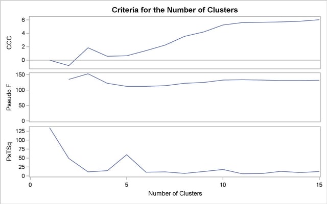
Figure 29.3 Plot of Statistics for Estimating the Number of Clusters

To interpret the values of the pseudo $\text{[math]}$ statistic, look down the column or look at the plot from right to left until you find the first value markedly larger than the previous value, then move back up the column or to the right in the plot by one step in the cluster history. In Figure 29.3, you can see possibly good clustering levels at 11 clusters, 6 clusters, 3 clusters, and 2 clusters.

Considered together, these statistics suggest that the data can be clustered into 11 clusters or 3 clusters. The following statements examine the results of clustering the data into 3 clusters.

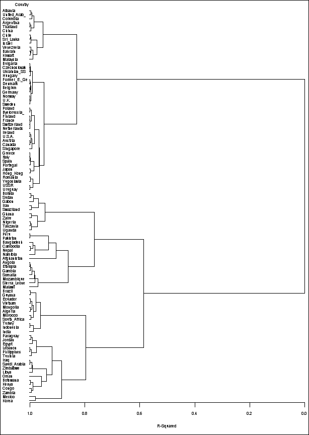
A graphical view of the clustering process can often be helpful in interpreting the clusters. The following statements use the TREE procedure to produce a tree diagram of the clusters:

   goptions vsize=9in hsize=6.4in htext=.9pct htitle=3pct;
   axis1 order=(0 to 1 by 0.2);
   proc tree data=Tree out=New nclusters=3
             haxis=axis1 horizontal;
      height _rsq_;
      copy can1 can2 ;
      id country;
   run;

The AXIS1 statement defines axis parameters that are used in the TREE procedure. The ORDER= option specifies the data values in the order in which they should appear on the axis.

The preceding statements use the SAS data set Tree as input. The OUT= option creates an output SAS data set named New to contain information about cluster membership. The NCLUSTERS= option specifies the number of clusters desired in the data set New.

The TREE procedure produces high-resolution graphics by default. The HAXIS= option specifies AXIS1 to customize the appearance of the horizontal axis. The HORIZONTAL option orients the tree diagram horizontally. The HEIGHT statement specifies the variable _RSQ_ (R square) as the height variable.

The COPY statement copies the canonical variables can1 and can2 (computed in the ACECLUS procedure) into the output SAS data set New. Thus, the SAS output data set New contains information for three clusters and the first two of the original canonical variables.

Figure 29.4 displays the tree diagram. The figure provides a graphical view of the information in Figure 29.2. As the number of branches grows to the left from the root, the R square approaches 1; the first three clusters (branches of the tree) account for over half of the variation (about 77%, from Figure 29.4). In other words, only three clusters are necessary to explain over three-fourths of the variation.

Figure 29.4 Tree Diagram of Clusters versus R-Square Values

The following statements invoke the SGPLOT procedure on the SAS data set New:

   proc sgplot data=New ;
      scatter y=can2 x=can1 / group=cluster ;
   run;

The PLOT statement requests a plot of the two canonical variables, using the value of the variable cluster as the identification variable, as shown in Figure 29.5.

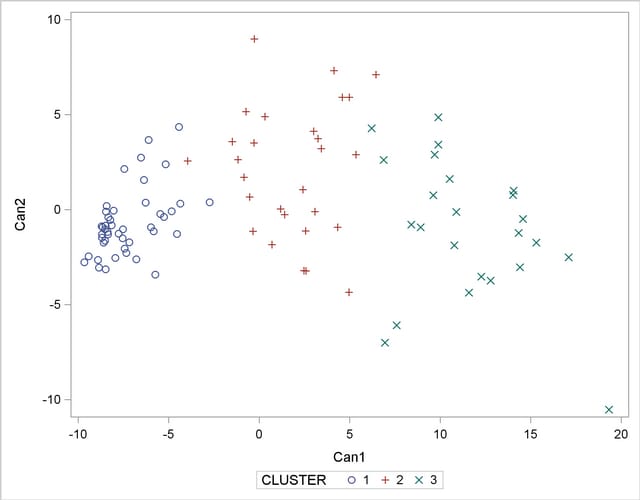
Figure 29.5 Plot of Canonical Variables and Cluster for Three Clusters

The statistics in Figure 29.2 and Figure 29.3, the tree diagram in Figure 29.4, and the plot of the canonical variables in Figure 29.5 assist in the estimation of clusters in the data. There seems to be reasonable separation in the clusters. However, you must use this information, along with experience and knowledge of the field, to help in deciding the correct number of clusters.

Footnotes

These data have been compiled from the United Nations Demographic Yearbook 1990 (United Nations publications, Sales No. E/F.91.XII.1, copyright 1991, United Nations, New York) and are reproduced with the permission of the United Nations.

Top of Page