specifies the significance level for a confidence interval, , for the Browne and Cudeck (1993) expected cross validation index (ECVI). The default value is , which corresponds to a 90% confidence interval for the ECVI.

specifies the significance level for a confidence interval, , for the Steiger and Lind (1980) root mean squared error of approximation (RMSEA) coefficient (refer to Browne and Du Toit 1992). The default value is , which corresponds to a 90% confidence interval for the RMSEA.

specifies an absolute singularity criterion , , for the inversion of the information matrix, which is needed to compute the covariance matrix. The following singularity criterion is used:

In the preceding criterion, is the diagonal pivot of the matrix, and VSING and MSING are the specified values of the VSINGULAR= and MSINGULAR= options. The default value for ASING is the square root of the smallest positive double-precision value. Note that, in many cases, a normalized matrix is decomposed, and the singularity criteria are modified correspondingly.

specifies the formula for asymptotic covariances used in the weight matrix for WLS and DWLS estimation. The ASYCOV option is effective only if METHOD=WLS or METHOD=DWLS and no INWGT= input data set is specified. The following formulas are implemented:

BIASED

Browne’s (1984) formula (3.4)
biased asymptotic covariance estimates; the resulting weight matrix is at least positive semidefinite. This is the default for analyzing a covariance matrix.

UNBIASED

Browne’s (1984) formula (3.8)
asymptotic covariance estimates corrected for bias; the resulting weight matrix can be indefinite (that is, can have negative eigenvalues), especially for small .

CORR

Browne and Shapiro’s (1986) formula (3.2), which is identical to DeLeeuw’s (1983) formulas (2, 3, 4)
the asymptotic variances of the diagonal elements are set to the reciprocal of the value specified by the WPENALTY= option (default: ). This formula is the default for analyzing a correlation matrix.

Caution:Using the WLS and DWLS methods with the ASYCOV=CORR option means that you are fitting a correlation (rather than a covariance) structure. Since the fixed diagonal of a correlation matrix for some models does not contribute to the model’s degrees of freedom, you can specify the DFREDUCE= option to reduce the degrees of freedom by the number of manifest variables used in the model. See the section Counting the Degrees of Freedom for more information.

analyzes the augmented correlation or covariance matrix. Using the AUG option is equivalent to specifying UCORR (NOINT but not COV) or UCOV (NOINT and COV) for a data set that is augmented by an intercept variable INTERCEPT that has constant values equal to 1. The variable INTERCEP can be used instead of the default INTERCEPT only if you specify the SAS option OPTIONS VALIDVARNAME=V6. The dimension of an augmented matrix is one higher than that of the corresponding correlation or covariance matrix. The AUGMENT option is effective only if the data set does not contain a variable called INTERCEPT and if you specify the UCOV, UCORR, or NOINT option.

Caution:The INTERCEPT variable is included in the moment matrix as the variable with number . Using the RAM model statement assumes that the first variable numbers correspond to the manifest variables in the input data set. Therefore, specifying the AUGMENT option assumes that the numbers of the latent variables used in the RAM or path model have to start with number .

computes univariate skewness and kurtosis by formulas uncorrected for bias. See the section Measures of Multivariate Kurtosis for more information.

analyzes the covariance matrix instead of the correlation matrix. By default, PROC CALIS (like the FACTOR procedure) analyzes a correlation matrix. If the DATA= input data set is a valid TYPE=CORR data set (containing a correlation matrix and standard deviations), using the COV option means that the covariance matrix is computed and analyzed.

specifies a nonnegative threshold , which determines whether the eigenvalues of the information matrix are considered to be zero. If the inverse of the information matrix is found to be singular (depending on the VSINGULAR=, MSINGULAR=, ASINGULAR=, or SINGULAR= option), a generalized inverse is computed using the eigenvalue decomposition of the singular matrix. Those eigenvalues smaller than are considered to be zero. If a generalized inverse is computed and you do not specify the NOPRINT option, the distribution of eigenvalues is displayed.

specifies an input data set that can be an ordinary SAS data set or a specially structured TYPE=CORR, TYPE=COV, TYPE=UCORR, TYPE=UCOV, TYPE=SSCP, or TYPE=FACTOR SAS data set, as described in the section Input Data Sets. If the DATA= option is omitted, the most recently created SAS data set is used.

changes the initial values of all parameters that are located on the diagonals of the central model matrices by the relationship

The initial values of the diagonal elements of the central matrices should always be nonnegative to generate positive-definite predicted model matrices in the first iteration. By using values of , such as , , ..., you can increase these initial values to produce predicted model matrices with high positive eigenvalues in the first iteration. The DEMPHAS= option is effective independently of the way the initial values are set; that is, it changes the initial values set in the model specification as well as those set by an INRAM= data set and those automatically generated for RAM, LINEQS, or FACTOR model statements. It also affects the initial values set by the START= option, which uses, by default, DEMPHAS=100 if a covariance matrix is analyzed and DEMPHAS=10 for a correlation matrix.

reduces the degrees of freedom of the test by . In general, the number of degrees of freedom is the number of elements of the lower triangle of the predicted model matrix , , minus the number of parameters, . If the NODIAG option is used, the number of degrees of freedom is additionally reduced by . Because negative values of are allowed, you can also increase the number of degrees of freedom by using this option. If the DFREDUCE= or NODIAG option is used in a correlation structure analysis, PROC CALIS does not additionally reduce the degrees of freedom by the number of constant elements in the diagonal of the predicted model matrix, which is otherwise done automatically. See the section Counting the Degrees of Freedom for more information.

makes the effective number of observations , where is 0 if the NOINT, UCORR, or UCOV option is specified without the AUGMENT option or where is 1 otherwise. You can also use the NOBS= option to specify the number of observations.

specifies the relative function convergence criterion. The optimization process is terminated when the relative difference of the function values of two consecutive iterations is smaller than the specified value of ; that is,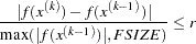

where can be defined by the FSIZE= option in the NLOPTIONS statement.

The default value is , where either can be specified in the NLOPTIONS statement or is set by default to , where is the machine precision.

replaces the analytic derivatives of the programming statements by numeric derivatives (finite-difference approximations). In general, this option is needed only when you have programming statements that are too difficult for the built-in function compiler to differentiate analytically. For example, if the program code for the nonlinear constraints contains many arrays and many DO loops with array processing, the built-in function compiler can require too much time and memory to compute derivatives of the constraints with respect to the parameters. In this case, the Jacobian matrix of constraints is computed numerically by using finite-difference approximations. The FDCODE option does not modify the kind of derivatives specified with the HESSALG= option.

specifies the algorithm to compute the approximate covariance matrix of parameter estimates used for computing the approximate standard errors and modification indices when the information matrix is singular. If the number of parameters used in the model you analyze is smaller than the value of , the time-expensive Moore-Penrose (G4) inverse of the singular information matrix is computed by eigenvalue decomposition. Otherwise, an inexpensive pseudo (G1) inverse is computed by sweeping. By default, . For more details, see the section Estimation Criteria.

specifies the relative gradient convergence criterion (see the ABSGCONV= option for the absolute gradient convergence criterion).

Termination of all techniques (except the CONGRA technique) requires the normalized predicted function reduction to be small,

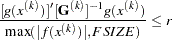
where can be defined by the FSIZE= option in the NLOPTIONS statement. For the CONGRA technique (where a reliable Hessian estimate is not available),

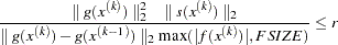
is used. The default value is .

Note that prior to SAS 6.11, the GCONV= option specified the absolute gradient convergence criterion.

specifies the algorithm used to compute the (approximate) Hessian matrix when TECHNIQUE=LEVMAR and NEWRAP, to compute approximate standard errors of the parameter estimates, and to compute Lagrange multipliers. There are different groups of algorithms available:

• analytic formulas: HA=1,2,3,4,11

• finite-difference approximation: HA=5,6

• dense storage: HA=1,2,3,4,5,6

• sparse storage: HA=11

If the Jacobian is more than 25% dense, the dense analytic algorithm, HA, is used by default. The HA algorithm is faster than the other dense algorithms, but it needs considerably more memory for large problems than HA,,. If the Jacobian is more than 75% sparse, the sparse analytic algorithm, HA, is used by default. The dense analytic algorithm HA corresponds to the original COSAN algorithm; you are advised not to specify HA due to its very slow performance. If there is not enough memory available for the dense analytic algorithm HA and you must specify HA or HA, it might be more efficient to use one of the quasi-Newton or conjugate-gradient optimization techniques since Levenberg-Marquardt and Newton-Raphson optimization techniques need to compute the Hessian matrix in each iteration. For approximate standard errors and modification indices, the Hessian matrix has to be computed at least once, regardless of the optimization technique.

The algorithms HA and HA compute approximate derivatives by using forward-difference formulas. The HA algorithm corresponds to the analytic HA: it is faster than HA, but it needs much more memory. The HA algorithm corresponds to the analytic HA: it is slower than HA, but it needs much less memory.

Test computations of large sparse problems show that the sparse algorithm HA can be up to 10 times faster than HA (and needs much less memory).

specifies an input data set that contains initial estimates for the parameters used in the optimization process and can also contain boundary and general linear constraints on the parameters. If the model did not change too much, you can specify an OUTEST= data set from a previous PROC CALIS analysis. The initial estimates are taken from the values of the PARMS observation.

specifies an input data set that contains in RAM list form all information needed to specify an analysis model. The INRAM= data set is described in the section Input Data Sets. Typically, this input data set is an OUTRAM= data set (possibly modified) from a previous PROC CALIS analysis. If you use an INRAM= data set to specify the analysis model, you cannot use the model specification statement COSAN, MATRIX, RAM, LINEQS, STD, COV, FACTOR, or VARNAMES, but you can use the BOUNDS and PARAMETERS statements and programming statements. If the INRAM= option is omitted, you must define the analysis model with a COSAN, RAM, LINEQS, or FACTOR statement.

For highly nonlinear objective functions, such as the EXP function, the default initial radius of the trust-region algorithms TRUREG, DBLDOG, and LEVMAR or the default step length of the line-search algorithms can produce arithmetic overflows. If this occurs, specify decreasing values of such as INSTEP=1E1, INSTEP=1E2, INSTEP=1E4, ..., until the iteration starts successfully.

• For trust-region algorithms (TRUREG, DBLDOG, and LEVMAR), the INSTEP option specifies a positive factor for the initial radius of the trust-region. The default initial trust-region radius is the length of the scaled gradient, and it corresponds to the default radius factor of .

• For line-search algorithms (NEWRAP, CONGRA, and QUANEW), INSTEP specifies an upper bound for the initial step length for the line search during the first five iterations. The default initial step length is .

For releases prior to SAS 6.11, specify the SALPHA= and RADIUS= options. For more details, see the section Computational Problems.

specifies an input data set that contains the weight matrix used in generalized least squares (GLS), weighted least squares (WLS, ADF), or diagonally weighted least squares (DWLS) estimation. If the weight matrix defined by an INWGT= data set is not positive-definite, it can be ridged by using the WRIDGE= option. See the section Estimation Criteria for more information. If no INWGT= data set is specified, default settings for the weight matrices are used in the estimation process. The INWGT= data set is described in the section Input Data Sets. Typically, this input data set is an OUTWGT= data set from a previous PROC CALIS analysis.

computes and displays univariate kurtosis and skewness, various coefficients of multivariate kurtosis, and the numbers of observations that contribute most to the normalized multivariate kurtosis. See the section Measures of Multivariate Kurtosis for more information. Using the KURTOSIS option implies the SIMPLE display option. This information is computed only if the DATA= data set is a raw data set, and it is displayed by default if the PRINT option is specified. The multivariate LS kappa and the multivariate mean kappa are displayed only if you specify METHOD=WLS and the weight matrix is computed from an input raw data set. All measures of skewness and kurtosis are corrected for the mean. If an intercept variable is included in the analysis, the measures of multivariate kurtosis do not include the intercept variable in the corrected covariance matrix, as indicated by a displayed message. Using the BIASKUR option displays the biased values of univariate skewness and kurtosis.

specifies the line-search method for the CONGRA, QUANEW, and NEWRAP optimization techniques. Refer to Fletcher (1980) for an introduction to line-search techniques. The value of can be ; the default is .

LIS=1

specifies a line-search method that needs the same number of function and gradient calls for cubic interpolation and cubic extrapolation; this method is similar to one used by the Harwell subroutine library.

LIS=2

specifies a line-search method that needs more function calls than gradient calls for quadratic and cubic interpolation and cubic extrapolation; this method is implemented as shown in Fletcher (1987) and can be modified to an exact line search by using the LSPRECISION= option.

LIS=3

specifies a line-search method that needs the same number of function and gradient calls for cubic interpolation and cubic extrapolation; this method is implemented as shown in Fletcher (1987) and can be modified to an exact line search by using the LSPRECISION= option.

LIS=4

specifies a line-search method that needs the same number of function and gradient calls for stepwise extrapolation and cubic interpolation.

LIS=5

specifies a line-search method that is a modified version of LIS=4.

LIS=6

specifies golden section line search (Polak 1971), which uses only function values for linear approximation.

LIS=7

specifies bisection line search (Polak 1971), which uses only function values for linear approximation.

LIS=8

specifies Armijo line-search technique (Polak 1971), which uses only function values for linear approximation.

specifies the degree of accuracy that should be obtained by the line-search algorithms LIS=2 and LIS=3. Usually an imprecise line search is inexpensive and successful. For more difficult optimization problems, a more precise and more expensive line search might be necessary (Fletcher 1980, p. 22). The second (default for NEWRAP, QUANEW, and CONGRA) and third line-search methods approach exact line search for small LSPRECISION= values. If you have numerical problems, you should decrease the LSPRECISION= value to obtain a more precise line search. The default LSPRECISION= values are displayed in the following table.

For more details, refer to Fletcher (1980, pp. 25–29).

specifies the maximum number of function calls in the optimization process. The default values are displayed in the following table.

The default is used if you specify MAXFUNC=0. The optimization can be terminated only after completing a full iteration. Therefore, the number of function calls that are actually performed can exceed the number that is specified by the MAXFUNC= option.

specifies the maximum number of iterations in the optimization process. The default values are displayed in the following table.

The default is used if you specify MAXITER=0 or if you omit the MAXITER option.

The optional second value is valid only for TECH=QUANEW with nonlinear constraints. It specifies an upper bound for the number of iterations of an algorithm and reduces the violation of nonlinear constraints at a starting point. The default is =20. For example, specifying

   maxiter= . 0 

means that you do not want to exceed the default number of iterations during the main optimization process and that you want to suppress the feasible-point algorithm for nonlinear constraints.

specifies the method of parameter estimation. Valid values for name are as follows:

ML | M | MAX

performs normal-theory maximum likelihood parameter estimation. The ML method requires a nonsingular covariance or correlation matrix. This is the default method.

GLS | G

performs generalized least squares parameter estimation. If no INWGT= data set is specified, the GLS method uses the inverse sample covariance or correlation matrix as weight matrix . Therefore, METHOD=GLS requires a nonsingular covariance or correlation matrix.

WLS | W | ADF

performs weighted least squares parameter estimation. If no INWGT= data set is specified, the WLS method uses the inverse matrix of estimated asymptotic covariances of the sample covariance or correlation matrix as the weight matrix . In this case, the WLS estimation method is equivalent to Browne’s (1982, 1984) asymptotically distribution-free estimation. The WLS method requires a nonsingular weight matrix.

DWLS | D

performs diagonally weighted least squares parameter estimation. If no INWGT= data set is specified, the DWLS method uses the inverse diagonal matrix of asymptotic variances of the input sample covariance or correlation matrix as the weight matrix . The DWLS method requires a nonsingular diagonal weight matrix.

ULS | LS | U

performs unweighted least squares parameter estimation.

LSML | LSM | LSMAX

performs unweighted least squares followed by normal-theory maximum likelihood parameter estimation.

LSGLS | LSG

performs unweighted least squares followed by generalized least squares parameter estimation.

LSWLS | LSW | LSADF

performs unweighted least squares followed by weighted least squares parameter estimation.

LSDWLS | LSD

performs unweighted least squares followed by diagonally weighted least squares parameter estimation.

NONE | NO

uses no estimation method. This option is suitable for checking the validity of the input information and for displaying the model matrices and initial values.

The default estimation method is maximum likelihood (METHOD=ML), assuming a multivariate normal distribution of the observed variables. The two-stage estimation methods METHOD=LSML, METHOD=LSGLS, METHOD=LSWLS, and METHOD=LSDWLS first compute unweighted least squares estimates of the model parameters and their residuals. Afterward, these estimates are used as initial values for the optimization process to compute maximum likelihood, generalized least squares, weighted least squares, or diagonally weighted least squares parameter estimates. You can do the same thing by using an OUTRAM= data set with least squares estimates as an INRAM= data set for a further analysis to obtain the second set of parameter estimates. This strategy is also discussed in the section Use of Optimization Techniques. For more details, see the section Estimation Criteria.

computes and displays Lagrange multiplier test indices for constant parameter constraints, equality parameter constraints, and active boundary constraints, as well as univariate and multivariate Wald test indices. The modification indices are not computed in the case of unweighted or diagonally weighted least squares estimation.

The Lagrange multiplier test (Bentler 1986; Lee 1985; Buse 1982) provides an estimate of the reduction that results from dropping the constraint. For constant parameter constraints and active boundary constraints, the approximate change of the parameter value is displayed also. You can use this value to obtain an initial value if the parameter is allowed to vary in a modified model. For more information, see the section Modification Indices.

specifies a relative singularity criterion , , for the inversion of the information matrix, which is needed to compute the covariance matrix. The following singularity criterion is used:

where is the diagonal pivot of the matrix, and ASING and VSING are the specified values of the ASINGULAR= and VSINGULAR= options, respectively. If you do not specify the SINGULAR= option, the default value for MSING is 1E12; otherwise, the default value is 1E4 * SINGULAR. Note that, in many cases, a normalized matrix is decomposed, and the singularity criteria are modified correspondingly.

turns off the automatic adjustment of degrees of freedom when there are active constraints in the analysis. When the adjustment is in effect, most fit statistics and the associated probability levels will be affected. This option should be used when the researcher believes that the active constraints observed in the current sample will have little chance to occur in repeated sampling.

specifies the number of observations. If the DATA= input data set is a raw data set, nobs is defined by default to be the number of observations in the raw data set. The NOBS= and EDF= options override this default definition. You can use the RDF= option to modify the nobs specification. If the DATA= input data set contains a covariance, correlation, or scalar product matrix, you can specify the number of observations either by using the NOBS=, EDF=, and RDF= options in the PROC CALIS statement or by including a _TYPE_=’N’ observation in the DATA= input data set.

omits the diagonal elements of the analyzed correlation or covariance matrix from the fit function. This option is useful only for special models with constant error variables. The NODIAG option does not allow fitting of those parameters that contribute to the diagonal of the estimated moment matrix. The degrees of freedom are automatically reduced by . A simple example for the usefulness of the NODIAG option is the fit of the first-order factor model, . In this case, you do not have to estimate the diagonal matrix of unique variances that are fully determined by .

specifies that no intercept be used in computing covariances and correlations; that is, covariances or correlations are not corrected for the mean. You can specify this option (or UCOV or UCORR) to analyze mean structures in an uncorrected moment matrix—that is, to compute intercepts in systems of structured linear equations (see Example 25.2). The term NOINT is misleading in this case because an uncorrected covariance or correlation matrix is analyzed containing a constant (intercept) variable that is used in the analysis model. The degrees of freedom used in the variance divisor (specified by the VARDEF= option) and some of the assessment of the fit function (see the section Assessment of Fit) depend on whether an intercept variable is included in the model (the intercept is used in computing the corrected covariance or correlation matrix or is used as a variable in the uncorrected covariance or correlation matrix to estimate mean structures) or not included (an uncorrected covariance or correlation matrix is used that does not contain a constant variable).

does not compute modification indices. The NOMOD option is useful in connection with the PALL option because it saves computing time.

suppresses the displayed output. Note that this option temporarily disables the Output Delivery System (ODS). For more information, see Chapter 20, Using the Output Delivery System.

specifies that standard errors should not be computed. Standard errors are not computed for unweighted least squares (ULS) or diagonally weighted least squares (DWLS) estimation. In general, standard errors are computed even if the STDERR display option is not used (for file output).

creates an output data set containing the parameter estimates, their gradient, Hessian matrix, and boundary and linear constraints. For METHOD=ML, METHOD=GLS, and METHOD=WLS, the OUTEST= data set also contains the information matrix, the approximate covariance matrix of the parameter estimates ((generalized) inverse of information matrix), and approximate standard errors. If linear or nonlinear equality or active inequality constraints are present, the Lagrange multiplier estimates of the active constraints, the projected Hessian, and the Hessian of the Lagrange function are written to the data set. The OUTEST= data set also contains the Jacobian if the OUTJAC option is used.

The OUTEST= data set is described in the section OUTEST= SAS-data-set. If you want to create a permanent SAS data set, you must specify a two-level name. Refer to the chapter titled "SAS Data Files" in SAS Language Reference: Concepts for more information about permanent data sets.

writes the Jacobian matrix, if it has been computed, to the OUTEST= data set. This is useful when the information and Jacobian matrices need to be computed for other analyses.

creates an output data set containing the model information for the analysis, the parameter estimates, and their standard errors. An OUTRAM= data set can be used as an input INRAM= data set in a subsequent analysis by PROC CALIS. The OUTRAM= data set also contains a set of fit indices; it is described in more detail in the section OUTRAM= SAS-data-set. If you want to create a permanent SAS data set, you must specify a two-level name. Refer to the chapter titled "SAS Data Files" in SAS Language Reference: Concepts for more information about permanent data sets.

creates an output data set containing the BY-group variables, the analyzed covariance or correlation matrices, and the predicted and residual covariance or correlation matrices of the analysis. You can specify the correlation or covariance matrix in an OUTSTAT= data set as an input DATA= data set in a subsequent analysis by PROC CALIS. The OUTSTAT= data set is described in the section OUTSTAT= SAS-data-set. If the model contains latent variables, this data set also contains the predicted covariances between latent and manifest variables and the latent variable score regression coefficients (see the PLATCOV option). If the FACTOR statement is used, the OUTSTAT= data set also contains the rotated and unrotated factor loadings, the unique variances, the matrix of factor correlations, the transformation matrix of the rotation, and the matrix of standardized factor loadings.

You can use the latent variable score regression coefficients with PROC SCORE to compute latent variable or factor scores. For details, see the section Latent Variable Scores.

If you want to create a permanent SAS data set, you must specify a two-level name. Refer to the chapter titled "SAS Data Files" in SAS Language Reference: Concepts for more information about permanent data sets.

creates an output data set containing the weight matrix used in the estimation process. You cannot create an OUTWGT= data set with an unweighted least squares or maximum likelihood estimation. The fit function in GLS, WLS (ADF), and DWLS estimation contains the inverse of the (Cholesky factor of the) weight matrix written in the OUTWGT= data set. The OUTWGT= data set contains the weight matrix to which the WRIDGE= and the WPENALTY= options are applied. An OUTWGT= data set can be used as an input INWGT= data set in a subsequent analysis by PROC CALIS. The OUTWGT= data set is described in the section OUTWGT= SAS-data-set. If you want to create a permanent SAS data set, you must specify a two-level name. Refer to the chapter titled "SAS Data Files" in SAS Language Reference: Concepts for more information about permanent data sets.

displays all optional output except the output generated by the PCOVES, PDETERM, PJACPAT, and PRIVEC options.

Caution:The PALL option includes the very expensive computation of the modification indices. If you do not really need modification indices, you can save computing time by specifying the NOMOD option in addition to the PALL option.

displays the (corrected or uncorrected) covariance or correlation matrix that is analyzed and the predicted model covariance or correlation matrix.

displays the following:

• the information matrix (crossproduct Jacobian)

• the approximate covariance matrix of the parameter estimates (generalized inverse of the information matrix)

• the approximate correlation matrix of the parameter estimates

The covariance matrix of the parameter estimates is not computed for the ULS and DWLS estimation methods. This displayed output is not included in the output generated by the PALL option.

displays three coefficients of determination: the determination of all equations (DETAE), the determination of the structural equations (DETSE), and the determination of the manifest variable equations (DETMV). These determination coefficients are intended to be global means of the squared multiple correlations for different subsets of model equations and variables. The coefficients are displayed only when you specify a RAM or LINEQS model, but they are displayed for all five estimation methods: ULS, GLS, ML, WLS, and DWLS.

You can use the STRUCTEQ statement to define which equations are structural equations. If you do not use the STRUCTEQ statement, PROC CALIS uses its own default definition to identify structural equations.

The term "structural equation" is not defined in a unique way. The LISREL program defines the structural equations by the user-defined BETA matrix. In PROC CALIS, the default definition of a structural equation is an equation that has a dependent left-side variable that appears at least once on the right side of another equation, or an equation that has at least one right-side variable that is the left-side variable of another equation. Therefore, PROC CALIS sometimes identifies more equations as structural equations than the LISREL program does.

If the model contains structural equations, PROC CALIS also displays the "Stability Coefficient of Reciprocal Causation"—that is, the largest eigenvalue of the matrix, where is the causal coefficient matrix of the structural equations. These coefficients are computed as in the LISREL VI program of Jöreskog and Sörbom (1985). This displayed output is not included in the output generated by the PALL option.

displays the parameter estimates. In some cases, this includes displaying the standard errors and values.

displays the input model matrices and the vector of initial values.

displays the structure of variable and constant elements of the Jacobian matrix. This displayed output is not included in the output generated by the PALL option.

displays the following:

• the estimates of the covariances among the latent variables

• the estimates of the covariances between latent and manifest variables

• the latent variable score regression coefficients

The estimated covariances between latent and manifest variables and the latent variable score regression coefficients are written to the OUTSTAT= data set. You can use the score coefficients with PROC SCORE to compute factor scores. For details, see the section Latent Variable Scores.

specifies the ODS graphical plots. Currently, the only available ODS graphical plots in PROC CALIS are for residual distributions. Also, when the residual histograms are requested, the bar charts of residual tallies are suppressed. To display these bar charts with the residual histograms, you must use the RESIDUAL(TALLY) option.

When you specify only one plot-request, you can omit the parentheses around the plot-request. For example:

   plots=all
   plots=residuals

You must enable ODS Graphics before requesting plots; for example:

   ods graphics on;
   
   proc calis plots=residuals;
   run;
   
   ods graphics off;

For more information about the ODS GRAPHICS statement, see Chapter 21, Statistical Graphics Using ODS.

The following table shows the available plot-requests:

displays the pattern of variable and constant elements of the predicted moment matrix that is predetermined by the analysis model. It is especially helpful in finding manifest variables that are not used or that are used as exogenous variables in a complex model specified in the COSAN statement. Those entries of the predicted moment matrix for which the model generates variable (rather than constant) elements are displayed as missing values. This output is displayed even without specifying the PREDET option if the model generates constant elements in the predicted model matrix different from those in the analysis moment matrix and if you specify at least the PSHORT amount of displayed output.

If the analyzed matrix is a correlation matrix (containing constant elements of 1s in the diagonal) and the model generates a predicted model matrix with constant (rather than variable) elements in the diagonal, the degrees of freedom are automatically reduced by . The output generated by the PREDET option displays those constant diagonal positions. If you specify the DFREDUCE= or NODIAG option, this automatic reduction of the degrees of freedom is suppressed. See the section Counting the Degrees of Freedom for more information.

displays parameter estimates, approximate standard errors, and t values in matrix form if you specify the analysis model in the RAM or LINEQS statement. When a COSAN statement is used, this occurs by default.

adds the options KURTOSIS, RESIDUAL, PLATCOV, and TOTEFF to the default output.

displays parameter estimates, approximate standard errors, the gradient, and t values in vector form. The values are displayed with more decimal places. This displayed output is not included in the output generated by the PALL option.

excludes the output produced by the PINITIAL, SIMPLE, and STDERR options from the default output.

displays the fit assessment table and the ERROR, WARNING, and NOTE messages.

displays the weight matrix used in the estimation. The weight matrix is displayed after the WRIDGE= and WPENALTY= options are applied to it.

is an alias for the INSTEP= option for Levenberg-Marquardt minimization.

specifies a positive integer as a seed value for the pseudo-random number generator to generate initial values for the parameter estimates for which no other initial value assignments in the model definitions are made. Except for the parameters in the diagonal locations of the central matrices in the model, the initial values are set to random numbers in the range . The values for parameters in the diagonals of the central matrices are random numbers multiplied by or . For more information, see the section Initial Estimates.

makes the effective number of observations the actual number of observations minus the RDF= value. The degree of freedom for the intercept should not be included in the RDF= option. If you use PROC CALIS to compute a regression model, you can specify RDF= number-of-regressor-variables to get approximate standard errors equal to those computed by PROC REG.

displays the raw and normalized residual covariance matrices, the rank order of the largest residuals, and the bar charts of residual tallies. This information is displayed by default when you specify the PRINT option.

Three types of normalized or standardized residual matrices can be chosen with the RESIDUAL= specification:

RESIDUAL= NORM

normalized residuals

RESIDUAL= VARSTAND  |  VARSTD

variance standardized residuals

RESIDUAL= ASYSTAND  |  ASYMSTD

asymptotically standardized residuals

When ODS graphical plots of residuals are also requested, the bar charts of residual tallies are suppressed. They are replaced with high-quality graphical histograms showing residual distributions. If you still want to display the bar charts in this situation, use the RESIDUAL(TALLY) or RESIDUAL(TALLY)= option.

For more details, see the section Assessment of Fit.

defines a ridge factor for the diagonal of the moment matrix that is analyzed. The matrix is transformed to

If you do not specify in the RIDGE option, PROC CALIS tries to ridge the moment matrix so that the smallest eigenvalue is about .

Caution:The moment matrix in the OUTSTAT= output data set does not contain the ridged diagonal.

is an alias for the INSTEP= option for line-search algorithms.

displays means, standard deviations, skewness, and univariate kurtosis if available. This information is displayed when you specify the PRINT option. If you specify the UCOV, UCORR, or NOINT option, the standard deviations are not corrected for the mean. If the KURTOSIS option is specified, the SIMPLE option is set by default.

specifies the singularity criterion , , used, for example, for matrix inversion. The default value is the square root of the relative machine precision or, equivalently, the square root of the largest double-precision value that, when added to 1, results in 1.

specifies the probability limit used for computing the stepwise multivariate Wald test. The process stops when the univariate probability is smaller than . The default value is .

is an alias for the LSPRECISION= option.

In general, this option is needed only in connection with the COSAN model statement, and it specifies a constant as an initial value for all the parameter estimates for which no other initial value assignments in the pattern definitions are made. Start values in the diagonal locations of the central matrices are set to if a COV or UCOV matrix is analyzed and if a CORR or UCORR matrix is analyzed. The default value is . Unspecified initial values in a FACTOR, RAM, or LINEQS model are usually computed by PROC CALIS. If none of the initialization methods are able to compute all starting values for a model specified by a FACTOR, RAM, or LINEQS statement, then the start values of parameters that could not be computed are set to , , or . If the DEMPHAS= option is used, the initial values of the diagonal elements of the central model matrices are multiplied by the value specified in the DEMPHAS= option. For more information, see the section Initial Estimates.

displays approximate standard errors if estimation methods other than unweighted least squares (ULS) or diagonally weighted least squares (DWLS) are used (and the NOSTDERR option is not specified). If you specify neither the STDERR nor the NOSTDERR option, the standard errors are computed for the OUTRAM= data set. This information is displayed by default when you specify the PRINT option.

specifies the optimization technique. Valid values for name are as follows:

CONGRA  |  CG

chooses one of four different conjugate-gradient optimization algorithms, which can be more precisely defined with the UPDATE= option and modified with the LINESEARCH= option. The conjugate-gradient techniques need only memory compared to the memory for the other three techniques, where is the number of parameters. On the other hand, the conjugate-gradient techniques are significantly slower than other optimization techniques and should be used only when memory is insufficient for more efficient techniques. When you choose this option, UPDATE=PB by default. This is the default optimization technique if there are more than 400 parameters to estimate.

DBLDOG | DD

performs a version of double-dogleg optimization, which uses the gradient to update an approximation of the Cholesky factor of the Hessian. This technique is, in many ways, very similar to the dual quasi-Newton method, but it does not use line search. The implementation is based on Dennis and Mei (1979) and Gay (1983).

LEVMAR | LM | MARQUARDT

performs a highly stable but, for large problems, memory- and time-consuming Levenberg-Marquardt optimization technique, a slightly improved variant of the Moré (1978) implementation. This is the default optimization technique if there are fewer than 40 parameters to estimate.

NEWRAP | NRA

performs a usually stable but, for large problems, memory- and time-consuming Newton-Raphson optimization technique. The algorithm combines a line-search algorithm with ridging, and it can be modified with the LINESEARCH= option. Prior to SAS 6.11, this option invokes the NRRIDG option.

NRRIDG | NRR | NR | NEWTON

performs a usually stable but, for large problems, memory- and time-consuming Newton-Raphson optimization technique. This algorithm does not perform a line search. Since TECH=NRRIDG uses an orthogonal decomposition of the approximate Hessian, each iteration of TECH=NRRIDG can be slower than that of TECH=NEWRAP, which works with Cholesky decomposition. However, usually TECH=NRRIDG needs fewer iterations than TECH=NEWRAP.

QUANEW | QN

chooses one of four different quasi-Newton optimization algorithms that can be more precisely defined with the UPDATE= option and modified with the LINESEARCH= option. If boundary constraints are used, these techniques sometimes converge slowly. When you choose this option, UPDATE=DBFGS by default. If nonlinear constraints are specified in the NLINCON statement, a modification of Powell’s (1982a, 1982b) VMCWD algorithm is used, which is a sequential quadratic programming (SQP) method. This algorithm can be modified by specifying VERSION=1, which replaces the update of the Lagrange multiplier estimate vector to the original update of Powell (1978a, 1978b) that is used in the VF02AD algorithm. This can be helpful for applications with linearly dependent active constraints. The QUANEW technique is the default optimization technique if there are nonlinear constraints specified or if there are more than 40 and fewer than 400 parameters to estimate. The QUANEW algorithm uses only first-order derivatives of the objective function and, if available, of the nonlinear constraint functions.

TRUREG | TR

performs a usually very stable but, for large problems, memory- and time-consuming trust-region optimization technique. The algorithm is implemented similar to Gay (1983) and Moré and Sorensen (1983).

NONE | NO

does not perform any optimization. This option is similar to METHOD=NONE, but TECH=NONE also computes and displays residuals and goodness of fit statistics. If you specify METHOD=ML, METHOD=LSML, METHOD=GLS, METHOD=LSGLS, METHOD=WLS, or METHOD=LSWLS, this option enables computing and displaying (if the display options are specified) of the standard error estimates and modification indices corresponding to the input parameter estimates.

Since there is no single nonlinear optimization algorithm available that is clearly superior (in terms of stability, speed, and memory) for all applications, different types of optimization techniques are provided in the CALIS procedure. Each technique can be modified in various ways. The default optimization technique for fewer than 40 parameters () is TECHNIQUE=LEVMAR. For , TECHNIQUE=QUANEW is the default method, and for , TECHNIQUE=CONGRA is the default method. For more details, see the section Use of Optimization Techniques. You can specify the following set of options in the PROC CALIS statement or in the NLOPTIONS statement.

computes and displays total effects and indirect effects.

analyzes the uncorrected correlation matrix instead of the correlation matrix corrected for the mean. Using the UCORR option is equivalent to specifying the NOINT option but not the COV option.

analyzes the uncorrected covariance matrix instead of the covariance matrix corrected for the mean. Using the UCOV option is equivalent to specifying both the COV and NOINT options. You can specify this option to analyze mean structures in an uncorrected covariance matrix—that is, to compute intercepts in systems of linear structural equations (see Example 25.2).

specifies the update method for the quasi-Newton or conjugate-gradient optimization technique.

For TECHNIQUE=CONGRA, the following updates can be used:

PB

performs the automatic restart update method of Powell (1977) and Beale (1972). This is the default.

FR

performs the Fletcher-Reeves update (Fletcher 1980, p. 63).

PR

performs the Polak-Ribiere update (Fletcher 1980, p. 66).

CD

performs a conjugate-descent update of Fletcher (1987).

For TECHNIQUE=DBLDOG, the following updates (Fletcher 1987) can be used:

DBFGS

performs the dual Broyden-Fletcher-Goldfarb-Shanno (BFGS) update of the Cholesky factor of the Hessian matrix. This is the default.

DDFP

performs the dual Davidon-Fletcher-Powell (DFP) update of the Cholesky factor of the Hessian matrix.

For TECHNIQUE=QUANEW, the following updates (Fletcher 1987) can be used:

BFGS

performs original BFGS update of the inverse Hessian matrix. This is the default for earlier releases.

DFP

performs the original DFP update of the inverse Hessian matrix.

DBFGS

performs the dual BFGS update of the Cholesky factor of the Hessian matrix. This is the default.

DDFP

performs the dual DFP update of the Cholesky factor of the Hessian matrix.

specifies the divisor used in the calculation of covariances and standard deviations. The default value is VARDEF=DF. The values and associated divisors are displayed in the following table, where if the NOINT option is used and otherwise and where is the number of partial variables specified in the PARTIAL statement. Using an intercept variable in a mean structure analysis, by specifying the AUGMENT option, includes the intercept variable in the analysis. In this case, . When a WEIGHT statement is used, is the value of the WEIGHT variable in the th observation, and the summation is performed only over observations with positive weight.

specifies a relative singularity criterion , , for the inversion of the information matrix, which is needed to compute the covariance matrix. The following singularity criterion is used:

where is the diagonal pivot of the matrix, and ASING and MSING are the specified values of the ASINGULAR= and MSINGULAR= options. If you do not specify the SINGULAR= option, the default value for VSING is 1E8; otherwise, the default value is SINGULAR. Note that in many cases a normalized matrix is decomposed, and the singularity criteria are modified correspondingly.

specifies the penalty weight for the WLS and DWLS fit of the diagonal elements of a correlation matrix (constant 1s). The criterion for weighted least squares estimation of a correlation structure is

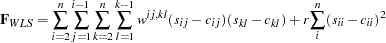
where is the penalty weight specified by the WPENALTY= option and the are the elements of the inverse of the reduced weight matrix that contains only the nonzero rows and columns of the full weight matrix . The second term is a penalty term to fit the diagonal elements of the correlation matrix. The default value is 100. The reciprocal of this value replaces the asymptotic variance corresponding to the diagonal elements of a correlation matrix in the weight matrix , and it is effective only with the ASYCOV=CORR option. The often used value seems to be too small in many cases to fit the diagonal elements of a correlation matrix properly. The default WPENALTY= value emphasizes the importance of the fit of the diagonal elements in the correlation matrix. You can decrease or increase the value of if you want to decrease or increase the importance of the diagonal elements fit. This option is effective only with the WLS or DWLS estimation method and the analysis of a correlation matrix. See the section Estimation Criteria for more details.

defines a ridge factor for the diagonal of the weight matrix used in GLS, WLS, or DWLS estimation. The weight matrix is transformed to

The WRIDGE= option is applied to the weight matrix as follows:

• before the WPENALTY= option is applied to it

• before the weight matrix is written to the OUTWGT= data set

• before the weight matrix is displayed