The following five estimation methods are available in PROC CALIS:

• unweighted least squares (ULS)

• generalized least squares (GLS)

• normal-theory maximum likelihood (ML)

• weighted least squares (WLS, ADF)

• diagonally weighted least squares (DWLS)

An INWGT= data set can be used to specify other than the default weight matrices for GLS, WLS, and DWLS estimation.

PROC CALIS do not exhaust all estimation methods in the field. As mentioned in the section Overview: CALIS Procedure, partial least squares (PLS) is not implemented. The PLS method is developed under less restrictive statistical assumptions. It circumvents some computational and theoretical problems encountered by the existing estimation methods in PROC CALIS. However, PLS estimates are less efficient in general. When the statistical assumptions of PROC CALIS are tenable (for example, large sample size, correct distributional assumptions, etc.), ML, GLS, or WLS methods yield better estimates than the PLS method. Note that there is a SAS/STAT procedure called PROC PLS, which employs the partial least squares technique but for a class of models different from those of PROC CALIS. For example, in a PROC CALIS model each latent variable is typically associated with only a subset of manifest variables (predictor or outcome variables). However, in PROC PLS latent variables are not prescribed with subsets of manifest variables. Rather, they are extracted from linear combinations of all manifest predictor variables. Therefore, for general path analysis with latent variables you should consider using PROC CALIS.

In each estimation method, the parameter vector is estimated iteratively by a nonlinear optimization algorithm that optimizes a goodness of fit function . When denotes the number of manifest variables, denotes the given sample covariance or correlation matrix for a sample with size , and denotes the predicted moment matrix, then the fit function for unweighted least squares estimation is

For normal-theory generalized least squares estimation, the function is

For normal-theory maximum likelihood estimation, the function is

The first three functions can be expressed by the generalized weighted least squares criterion (Browne 1982):

For unweighted least squares, the weight matrix is chosen as the identity matrix ; for generalized least squares, the default weight matrix is the sample covariance matrix ; and for normal-theory maximum likelihood, is the iteratively updated predicted moment matrix . The values of the normal-theory maximum likelihood function and the generally weighted least squares criterion with are asymptotically equivalent.

The goodness of fit function that is minimized in weighted least squares estimation is

where denotes the vector of the elements of the lower triangle of the symmetric matrix , and is a positive-definite symmetric matrix with rows and columns.

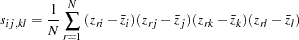
If the moment matrix is considered as a covariance rather than a correlation matrix, the default setting of is the consistent but biased estimators of the asymptotic covariances of the sample covariance with the sample covariance , as defined in the following:

where

The formula of the asymptotic covariances of uncorrected covariances (using the UCOV or NOINT option) is a straightforward generalization of this expression.

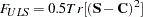
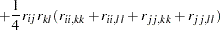
The resulting weight matrix is at least positive semidefinite (except for rounding errors). Using the ASYCOV option, you can use Browne’s (1984, formula (3.8)) unbiased estimators

There is no guarantee that this weight matrix is positive semidefinite. However, the second part is of order and does not destroy the positive semidefinite first part for sufficiently large . For a large number of independent observations, default settings of the weight matrix result in asymptotically distribution-free parameter estimates with unbiased standard errors and a correct test statistic (Browne 1982, 1984).

If the moment matrix is a correlation (rather than a covariance) matrix, the default setting of is the estimators of the asymptotic covariances of the correlations (Browne and Shapiro 1986; DeLeeuw 1983)

where

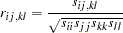The asymptotic variances of the diagonal elements of a correlation matrix are 0. Therefore, the weight matrix computed by Browne and Shapiro’s formula is always singular. In this case the goodness of fit function for weighted least squares estimation is modified to

where is the penalty weight specified by the WPENALTY= option and the are the elements of the inverse of the reduced weight matrix that contains only the nonzero rows and columns of the full weight matrix . The second term is a penalty term to fit the diagonal elements of the moment matrix . The default value of can be decreased or increased by the WPENALTY= option. The often used value of seems to be too small in many cases to fit the diagonal elements of a correlation matrix properly. If your model does not fit the diagonal of the moment matrix , you can specify the NODIAG option to exclude the diagonal elements from the fit function.

Storing and inverting the huge weight matrix in WLS estimation needs considerable computer resources. A compromise is found by implementing the DWLS method that uses only the diagonal of the weight matrix from the WLS estimation in the minimization function

The statistical properties of DWLS estimates are still not known.

In generalized, weighted, or diagonally weighted least squares estimation, you can change from the default settings of weight matrices by using an INWGT= data set. Because the diagonal elements of the weight matrix are interpreted as asymptotic variances of the sample covariances or correlations, they cannot be negative. The CALIS procedure requires a positive-definite weight matrix that has positive diagonal elements.